Archives
Mechanical Engineering Chapter 1 Homework Plot The Two Functions Sin And Versus
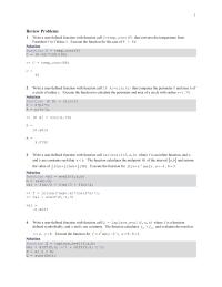
1 Review Problems 1. Write a user-defined function with function call C=temp_conv(F) that converts the temperature from Farenheit Fto Celsius C. Execute the function for the case of F = 86. Solution function C = temp_conv(F) C = (F-32)*100/180; 2. […]
Mechanical Engineering Chapter 10 Homework Figure 1059 Shows The Root Locus Unity
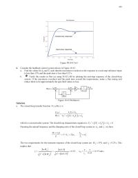
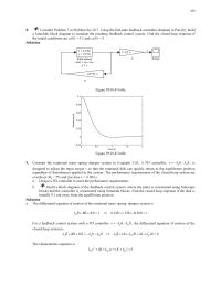
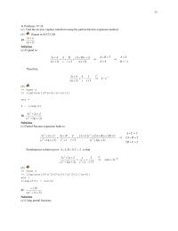
439 00.1 0.2 0.3 0.4 0.5 0.6 0.7 0.8 0 0.2 0.6 0.8 1 1.2 1.4 Step Response Time (sec) Figure PS10-4 No5 Amplitude Closed-loop response 6. Consider the feedback control system shown in Figure 10.43. a. Find the values […]
Mechanical Engineering Chapter 10 Homework Reconsider Example 106 Using The Final Value
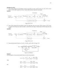
419 Problem Set 10.1 1. Draw a block diagram for the feedback control of a liquid-level system, which consists of a valve with a control knob (0–100%) and a liquid-level sensor. Clearly label essential components and signals. Solution 2. Draw […]
Mechanical Engineering Chapter 10 Homework Repeat Problem For The System Shown Figure
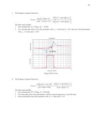
459 c. The frequency response function is 2 jȦMȦ 255 22 jȦMȦ 12 12 25 2 0.01 1 jȦ MȦ (jȦ jȦ MȦ 144 2 0.01 1 G ªº […]
Mechanical Engineering Chapter 10 Homework Thus The Gain Margin About
8. Consider Problem 7 in Problem Set 10.7. Using the full-state feedback controller obtained in Part (b), build a Simulink block diagram to simulate the resulting feedback control system. Find the closed-loop response if the initial conditions are x1(0) = […]
Mechanical Engineering Chapter 2 Homework Problems 3740 Evaluate X0 Using The Initial value
23 In Problems 19–24, (a) Find the inverse Laplace transform using the partial-fraction expansion method. (b) Repeat in MATLAB. 19. 34 (1) s ss Solution (a) Expand as 34 34 ( ) 41 (1) 1 (1) AB A […]
Mechanical Engineering Chapter 2 Homework Therefore, the six roots are
11 Problem Set 2.1 In Problems 1–4, (a) Perform 12 /zz and express the result in rectangular form, (b) Verify that 12 1 2 //zz z z , (c) Repeat Part (a)in MATLAB. 1.3 2 j j Solution (a) […]

Mechanical Engineering Chapter 3 Homework Find the row-echelon form and use it to determine the rank
35 Problem Set 3.1 In Problems 1–8 perform the indicated operations, if defined, for the vectors and matrices below. 0 30 2 1 0 1 , , , 1 12 15 4 2 3 ½ ªº ª º ½ […]
Mechanical Engineering Chapter 3 Homework Vav Expected Transformed Into Diagonal
50 5. 110 220 001 ªº «» «» «» ¬¼ A Solution (a) Block diagonal matrix; () 0,1,3 O A . For 10 O we solve >@ 111 110 0 1 2 2 0 0 1 001 0 0 […]
Mechanical Engineering Chapter 4 Homework A dynamic system with input f and output x is described by
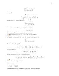
120 2 12 12 (2 1) 3 (3 2) 0 ss X X F XsX ° ® ° ¯ Solve for 1 X : 2. A dynamic system with input f and output x is described by […]
Mechanical Engineering Chapter 4 Homework Consequently The State Equation
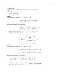
65 Problem Set 4.1 In Problems 1–10 express the system model, assuming general initial conditions, in (a) Configuration form, (b) Standard, second-order matrix form. 1. 11 12 1 22 12 2 2( ) 10 2( ) 0 t xx xx […]
Mechanical Engineering Chapter 4 Homework Electric charge q and electric current i are related
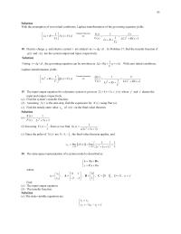
85 18. Electric charge qand electric current i are related via /idqdt . In Problem 17, find the transfer function if ()qt and ()vt are the system output and input, respectively. Solution Noting /idqdt , the governing equation can be […]
Mechanical Engineering Chapter 4 Homework Solution Step The Operating Point Satisfies 3
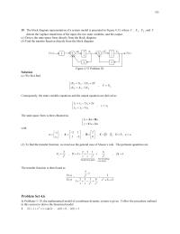
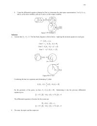
20. The block diagram representation of a system model is presented in Figure 4.33, where U, 1 X ,2 X , and Y denote the Laplace transforms of the input, the two state variables, and the output. (a) Derive the […]
Mechanical Engineering Chapter 5 Homework Applying The Moment Equation The Gives
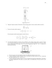
208 Figure Review5 No3 b. Taking the Laplace transform of both sides of the preceding equation with zero initial conditions results in 2 eq () 1 () Xs Fs ms k c. The state, the input, and the output […]
Mechanical Engineering Chapter 5 Homework Ignore The Control Force For Both Cases
194 b. Using the differential equation obtained in Part (a), determine the state–VSDFHUHSUHVHQWDWLRQ8VHșa,ș1Ȧa, DQGȦ1as tKHVWDWHYDULDEOHVDQGXVHș2DQGȦ2as the output variables. Figure 5.99 Problem 4. Solution a. Assume that a1 șș!! . The free-body diagram is shown below. Applying the moment equation to […]
Mechanical Engineering Chapter 5 Homework Rearranging The Equations Have X1 Figure
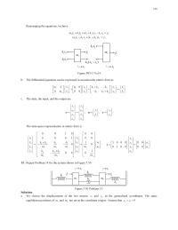
154 Rearranging the equations, we have 11 11 1 2 1 2 2 1 ()mx bx k k x k x f 22 21 2 3 2 2 ()mx kx k k x f b. The […]
Mechanical Engineering Chapter 5 Homework The free-body diagram of the system is shown
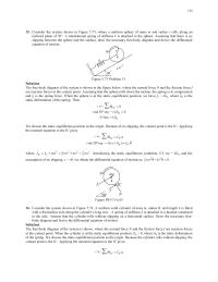
15. Consider the system shown in Figure 5.73, where a uniform sphere of mass mand radius rrolls along an inclined plane of 30°. A translational spring of stiffness kis attached to the sphere. Assuming that there is no slipping between […]
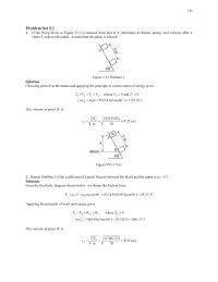
Mechanical Engineering Chapter 5 Homework The velocity at point B is
134 Problem Set 5.1 1. If the 50–kg block in Figure 5.12 is released from rest at A, determine its kinetic energy and velocity after it slides 5 m down the plane. Assume that the plane is smooth. Figure 5.12 […]
Mechanical Engineering Chapter 6 Homework Determine the equivalent resistance Req for the circuit
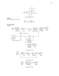
262 Figure 6.74 Problem 6. Solution The transfer function Vo(s)/Vi(s) is MATLAB Figures Problem 1 i(t) vC(t) V + – Voltage Sensor Switch f(x)=0 Solver Configuration Simulink–PS Converter Scope Re si st o r PS-Simulink Converter Electrical Reference DC Voltage […]
Mechanical Engineering Chapter 6 Homework Lcva Rcva Consider The Circuit Shown Figure
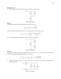
222 Problem Set 6.1 1. Determine the equivalent resistance Req for the circuit shown in Figure 6.8. Figure 6.8 Problem 1. Solution The equivalent resistance for the parallel-connected resistors R1and R3is eq1 1 3 111 RRR or 13 eq1 […]
Mechanical Engineering Chapter 6 Homework The op-amp circuit shown in Figure 6.39 is a non-inverting
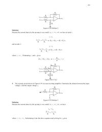
242 Figure 6.38 Problem 2. Solution Because the current drawn by the op-amp is very small, i.e., 0ii || , we have at node 1, 12 ii o 1 12 vv vv RR or 21 1o […]

Mechanical Engineering Chapter 6 Homework The State Equation And The Output Equation
274 which can be rearranged and gives the second equation 122 22 111 0vvv RRL or 1222 0Lv Lv R v b. Replacing the passive elements with their impedance representations gives the circuit in the sdomain […]
Mechanical Engineering Chapter 7 Homework Substituting These Expressions Results A2 Gh2 G
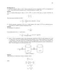
285 Problem Set 7.1 1. A car has an internal volume of 2.8 m3. If the sun heats the car from a temperature of 20°C to a temperature of 40°C, what will the pressure inside the car be? Assume the […]
Mechanical Engineering Chapter 7 Homework Write The Equations Secondorder Matrix Form Assume
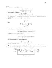
298 Solution a. The characteristic length of the junction is 3 4 body 3 c2 surface ʌ1 0.001 4ʌ Vr Lr Ar The Biot number of the junction is Thus, the junction can be treated as a lump-temperature system, […]
Mechanical Engineering Chapter 8 Homework Solution A Using And The Statespace Matrices
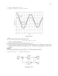
365 Figure PS8-5No11 12. A nonlinear dynamic system model is derived as 3 2 ( ) , (0) 0 , 0 3xxutx t dd where ()ut is the unit-step function. (a) Build the Simulink model and use it to […]
Mechanical Engineering Chapter 8 Homework Solution The Problem Formulated
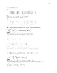
351 In Problems 5 through 10 determine the state vector via the formal-solution approach. 5. 21 1 0 , unit-step function , (0) 42 2 1 uu ªºªº ½ ®¾ «»«» ¬¼¬¼ ¯¿ xx x Solution […]
Mechanical Engineering Chapter 8 Homework Writing The Model Hand Standard Form Have
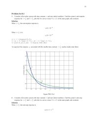
311 Problem Set 8.1 1. Consider a first-order system with time constant W and zero initial condition. Find the system’s unit-impulse response for 1 4 W and 1 2 W , plot the two curves versus 02tdd in the same […]
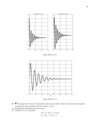
Mechanical Engineering Chapter 8 Homework The equations of motion of a mechanical system
331 Figure PS8-2No21-1 Figure PS8-2No21-2 22. The equations of motion of a mechanical system are given below, where ()t G denotes the unit-impulse. Assuming zero initial conditions, plot the response 1()xt by (a) Simulating the Simulink model of the system. […]
Mechanical Engineering Chapter 9 Homework An underdamped single-degree-of-freedom vibrating
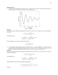
379 Problem Set 9.1 1. A lightly damped single-degree-of-freedom system is subjected to free vibration. The response of the system is shown in Figure (VWLPDWHWKHYDOXHRIWKHYLVFRXVGDPSLQJUDWLRȗ. Figure 9.5 Problem 1. Solution Note that the first and fifth peak displacements are about […]
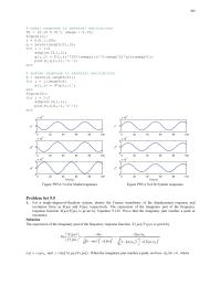
Mechanical Engineering Chapter 9 Homework Modal Response External Excitations 015 0
399 % modal response to external excitations f0 = [0.15 0 0]’; omega = 0.15; figure(1); 020 40 60 80 100 -5 020 40 60 80 100 -1 0 5x 10 1 0 1x 10 1 -5 q 020 40 […]