365
Figure PS8-5No11
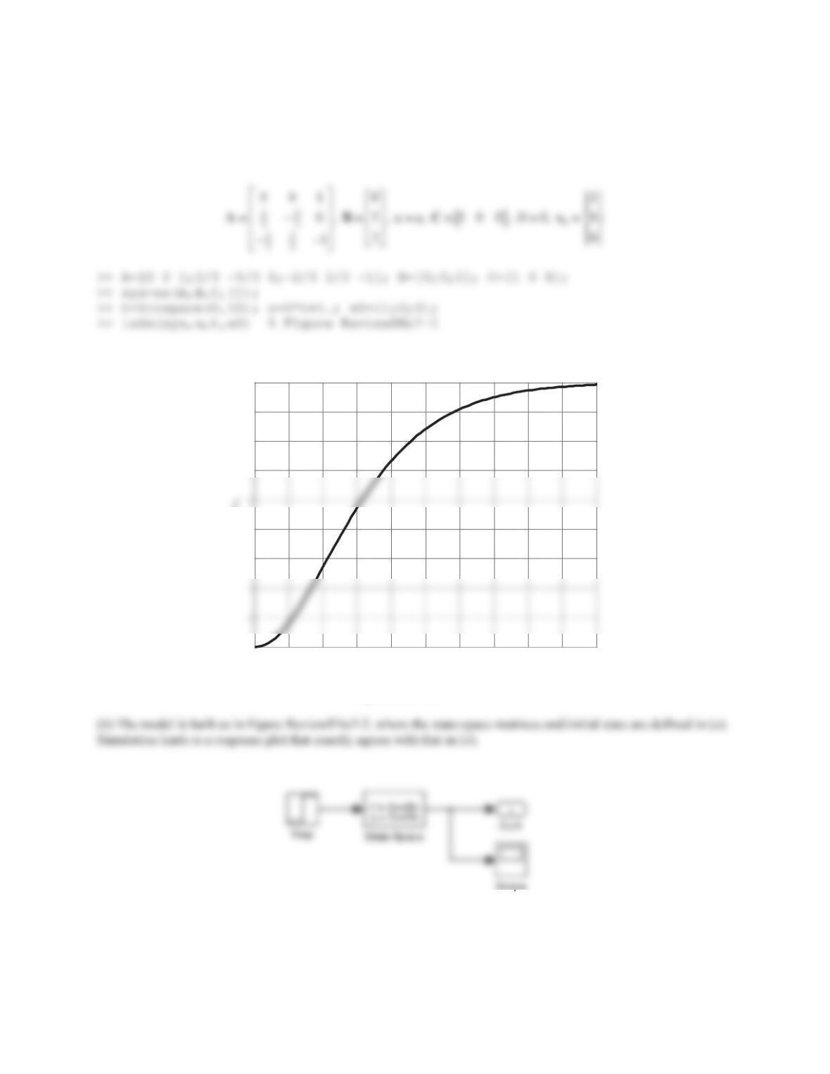
12. A nonlinear dynamic system model is derived as
3
2 ( ) , (0) 0 , 0 3xxutx t dd
where
()ut
is the unit-step function.
(a) Build the Simulink model and use it to generate the plot of
()xt
.
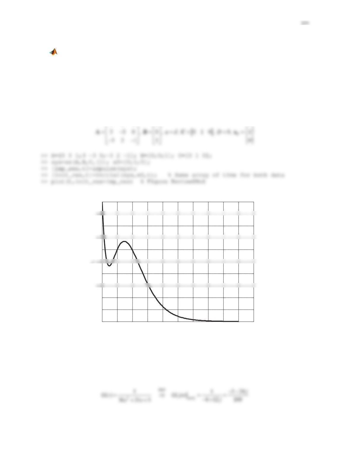
(b) Derive the linearized model analytically. Build a Simulink model and use it to plot the time variations of the
variable in the linear model that is compatible with
()xt
. Compare the plots generated in (a) and (b) and
comment.
Solution
(a) The model is built and shown in Figure PS8-5No12-1. Run the simulation, followed by
>> plot(tout,yout) % Figure PS8-5No12-2
00.5 11.5 22.5 33.5 44.5 5
-0.8
-0.4
0.2
0.4
Time
30 degrees
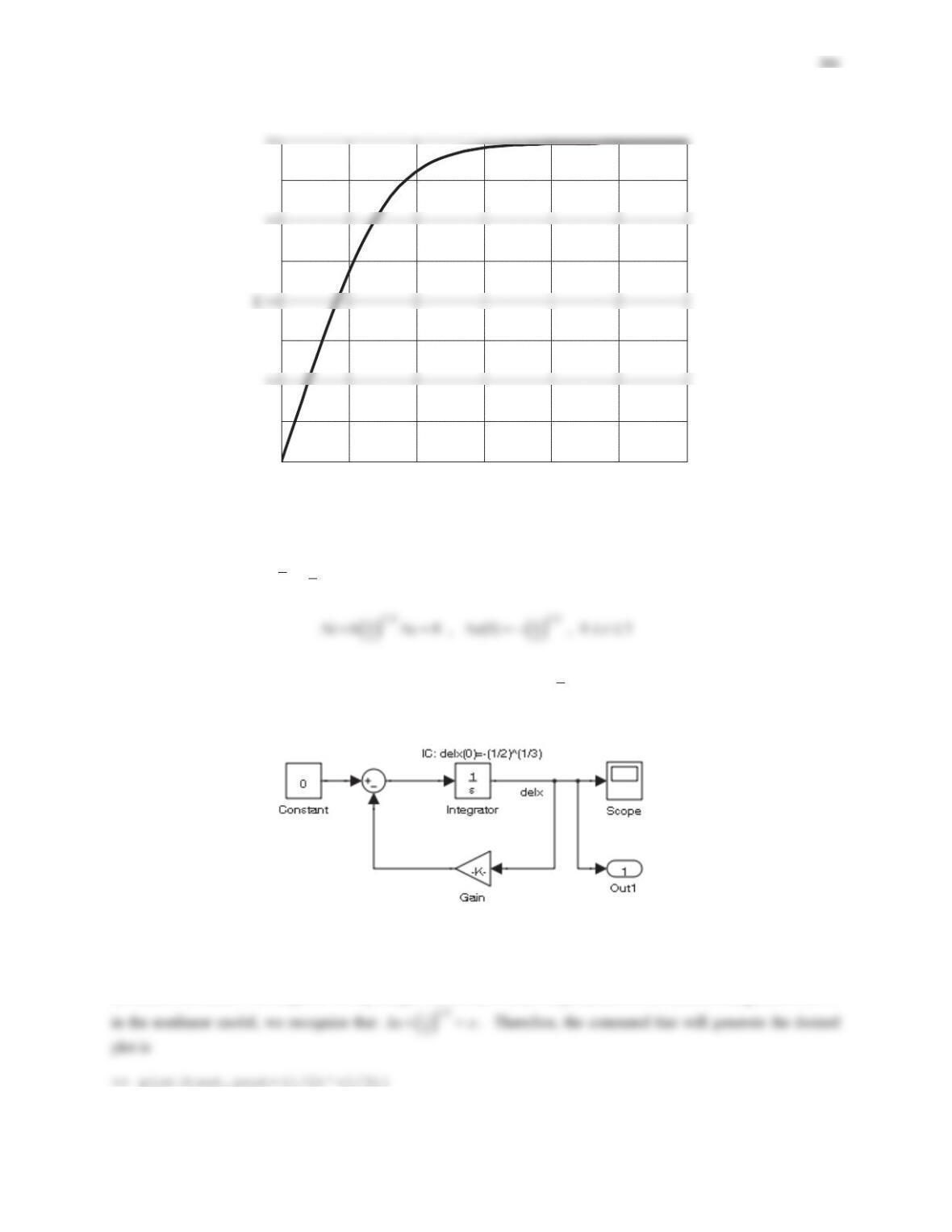
Figure PS8-5No12-2
(b) The operating point is
1/3
1
2
x
. The linearized model is derived as
The model is built as in Figure PS8-5No12-3, where the gain is
2/3
1
2
6K
.
Figure PS8-5No12-3
Simulate this model. The output is x‘by design. However, in order to get access to the variable compatible with
x
00.5 11.5 22.5 3
0
0.1
0.3
0.5
0.7
Time
367
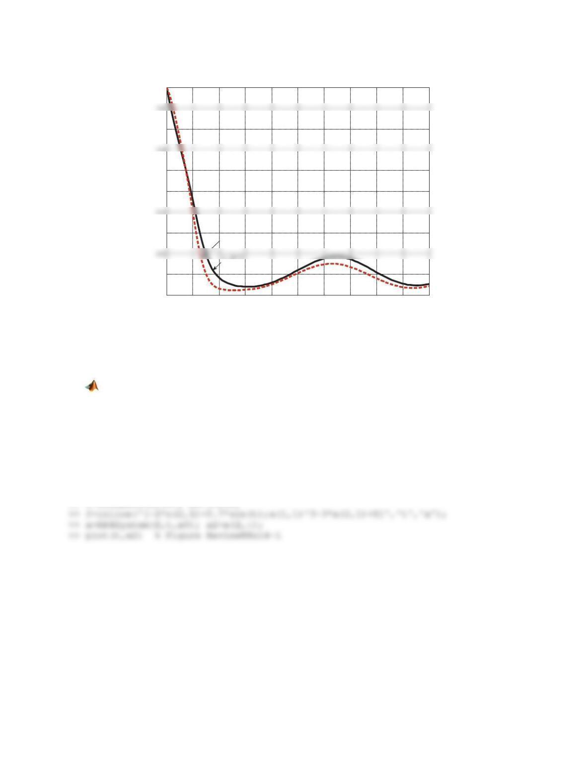
Embedding the plot generated in (a) into this new figure yields Figure PS8-5No12-4. As expected, the nonlinear and
linear responses agree near the operating point.
Figure PS8-5No12-4
Review Problems
1. A system is modeled as
1
2( ) 2 ( ) , (0) 0
r
yyutut y
where
()ut
and
()
r
ut
denote the unit-step and unit-ramp functions, respectively.
(a) Find the response
()yt
in closed form.
(b) Find and plot
()yt
,
010tdd
,usingthelsim command.
Solution
(a) In standard form,
22()4()
r
yy ut ut
so that 2
W
. Since the system is linear, we will use superposition to
find its total response. The response in
22()yy ut
is given by
00.5 11.5 22.5 3
0
0.1
0.3
0.5
0.7
Time
Linear
368
Figure Review8No1
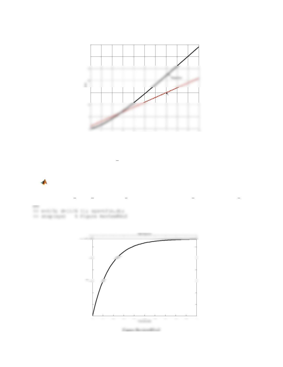
2. A first-order system is modeled as
1
2
3 2 ( ) , (0) 0yyut y
where
()ut
is the unit-step function.
(a) Determine the response
()yt
in closed form and find ss
y.
(b) Find and plot
()yt
using the step command.
Solution
(a) In standard form,
12
63
()yy ut
so that 1
6
W
. The response is given by
6
2
3
() 1
t
yt e
, hence
2
3
ss
y
.
15
30
35 Linear Simulation Results
Time (seconds)
Amplitude
Input
0
0.1
0.2
0.4
0.6
ss
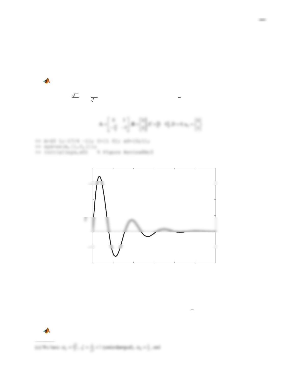
3. The model of a second-order system is given as
4 4 17 0 , (0) 0 , (0) 1xx x x x
(a) Identify the damping type and find the response in closed form.
(b) Find and plot the response using the initial command.
Solution
(a) We have
17 1
217
, 1 (underdamped), 2
nd
Z] Z
, and /2
1
2
() sin2
t
xt e t
.
(b) Using
1
xx
and
2
xx
, the state-space matrices are found as
Figure Review8No3
4. A second-order dynamic system is modeled as
1
2
9 12 5 10 ( ) , (0) 0 , (0)xxx tx x
G
(a) Find the response
()xt
in closed form.
(b) Find and plot the response using the impulse and initial commands.
02 4 6 8 10 12
-0.2
0.1
0.2
0.4
Response to Initial Conditions
Time (seconds)
370
(b) Using
1
xx
and
2
xx
, the state-space matrices are found as
Figure Review8No4
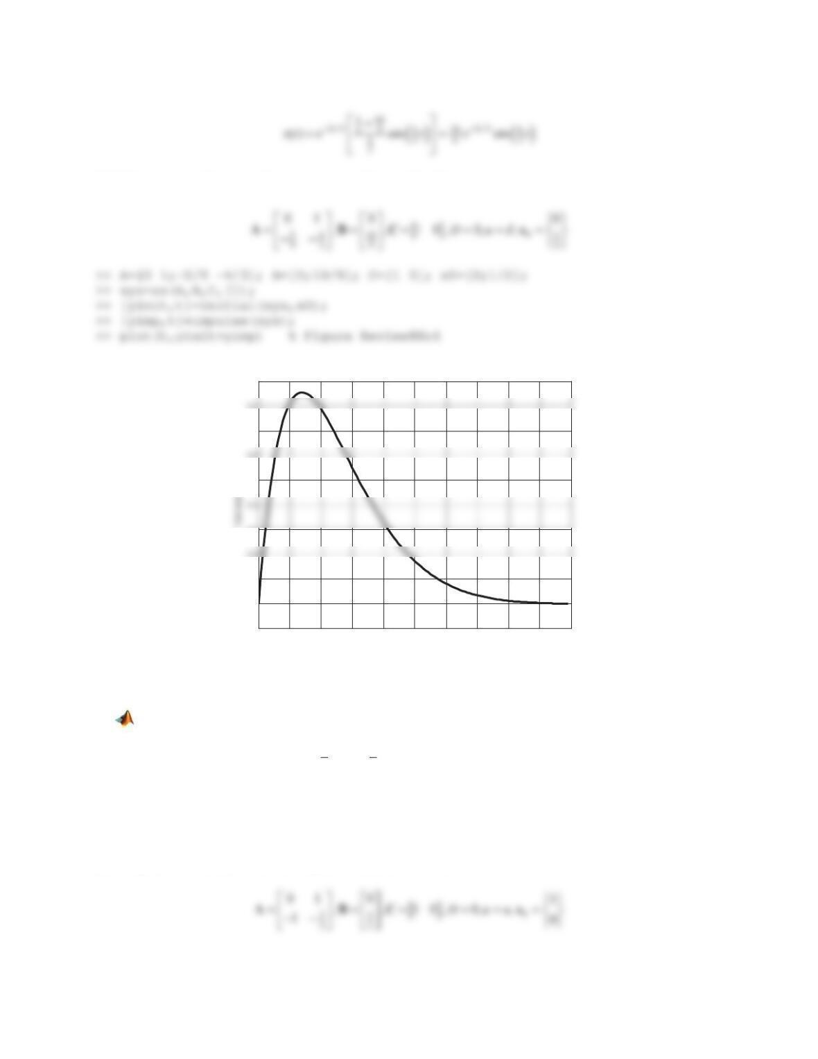
5. The mathematical model of a dynamic system is described by
35
22
( ) , (0) 1 , (0) 0xxxut x x
where
()ut
is the unit-step. Plot the response
()xt
by
(a)Using the initial and step commands.
(b) Simulating the Simulink model of the system.
Solution
(a) Using
1
xx
and
2
xx
, the state-space matrices are found as
0 1 2 3 4 5 6 7 8 9 10
-0.1
0
0.1
0.3
0.5
0.7
0.9
Time
371
>> A=[0 1;-1 -3/2]; B=[0;5/2]; C=[1 0]; x0=[1;0];
>> sys=ss(A,B,C,[]);
Figure Review8No5-1
(b) The model is built as in Figure Review8No5-2, where the state-space matrices and initial state are defined in (a).
Simulation leads to a response plot that exactly agrees with that in (a).
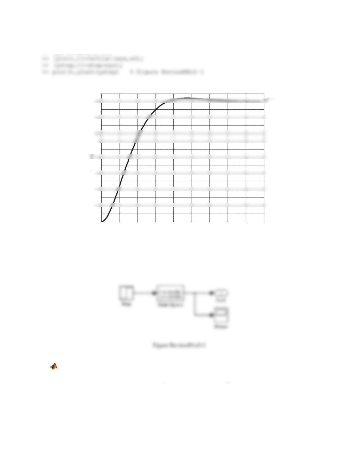
6. The mathematical model of a dynamic system is described by
11
32
4 4 5 ( ) , (0) 0 , (0)
r
xxx ut x x
where
()
r
ut
is the unit-ramp. Find and plot the response
()xt
by
(a)Using the lsim command over
05tdd
.
(b) Simulating the Simulink model of the system.
0123456789
1
1.1
1.3
1.5
1.7
1.9
2.2
2.4
2.6
Time
Total response
xss = 2.5
372
Solution
(a) Using
1
xx
and
2
xx
, the state-space matrices are found as
>@
0
511
412 2
01 0 0
,,10,0,,
1r
Duu
ªºªº ½
°°
®¾
«»«»
°°
¬¼¬¼ ¯¿
ABC x
Figure Review8No6-1
(b) The model is built as in Figure Review8No6-2, where the state-space matrices and initial state are defined in (a).
Simulation leads to a response plot that exactly agrees with that in (a).
Figure Review8No6-2
7. A dynamic system model is given as
2
11 21
3
12 1
2
22 21
3
()2()
, (0) 1, (0) 0, (0) 0
()5()
xx x x ut xx x
xx xx ut
°
®
°
¯
where
()ut
is the unit-step. Find and plot
1
x
,
010tdd
,by
00.5 11.5 22.5 33.5 44.5 5
1
1.5
4
4.5
5Linear Simulation Results
Time (seconds)
373
(a)Using the lsim command.
(b) Simulating the Simulink model of the system.
Solution
(a) With
112 231
, , xxx xxx
, the state-space matrices are obtained as
Figure Review8No7-1
Figure Review8No7-2
0 1 2 3 4 5 6 7 8 9 10
1
4
5
7
8
9
10 Linear Simulation Results
Time (seconds)
Amplitude x
8. The governing equations for a system are derived as
11 1 2
121
212
32 ()
, (0) 0, (0) 1, (0) 0
3 3 0
xx x x t xxx
xxx
G
®
¯
where
()t
G
is the unit-impulse. Find and plot 2
x,
010tdd
,using the impulse and initial commands.
Solution
With
112 231
, , xxx xxx
, the state-space matrices are obtained as
001 0 0
ªºªº ½
Figure Review8No8
9. Find the frequency response of a system whose model is
36 24 5 10sin( / 2)xxx t
.
Solution
The transfer function is
0 1 2 3 4 5 6 7 8 9 10
0
0.1
0.2
0.4
0.6
0.8
1
Time
x
375
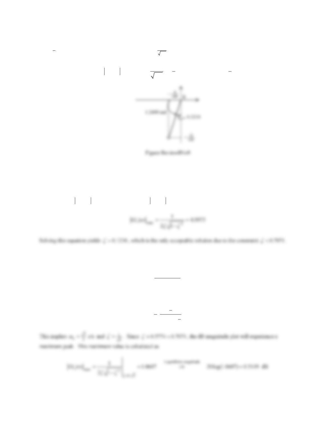
indicating a third quadrant location. The phase is therefore calculated as in Figure Review8No9, which yields
1
2
0.3218 1.8926 rad
IS
. The magnitude is
1
160
. Noting that 010F , we find
11
022
10
( ) ( ) sin( ) sin( 1.8926) 0.7906sin( 1.8926)
160
ss
xt FGj t t t
ZZI
10. Determine the damping ratio associated with a second-order system in the standard form of Eq. (8.32) that
corresponds to a maximum logarithmic magnitude of
12.25 dB
.
Solution
We have
max
20log ( ) 14.0231 dBGj
Z
, hence
max
( ) 4.0973Gj
Z
. Therefore,
11. Decide whether the magnitude (dB) plot for the following transfer function attains a maximum peak. If so,
calculate the maximum value and the corresponding frequency.
2
1
443ss
Solution
The transfer function is rewritten as
3
4
23
4
1
3ss
376
12. The state-space form of a system model is given as
®
¯
xAxBu
yCx
where
0
101 00 0
100
0 2 1 , 1 0 , , , 1
001 2
002 01 1
t
e
ªºªº ½
½
ªº
°° °°
«»«»
®¾ ®¾
«»
«»«» °°
¬¼ °°
¯¿
«»«»
¬¼¬¼ ¯¿
ABCux
Find the output vector yusing the formal solution of the state vector.
Solution
>> A=[1 0 1;0 -2 1;0 0 2]; B=[0 0;1 0;0 1]; C=[1 0 0;0 0 1];
>> syms t tau
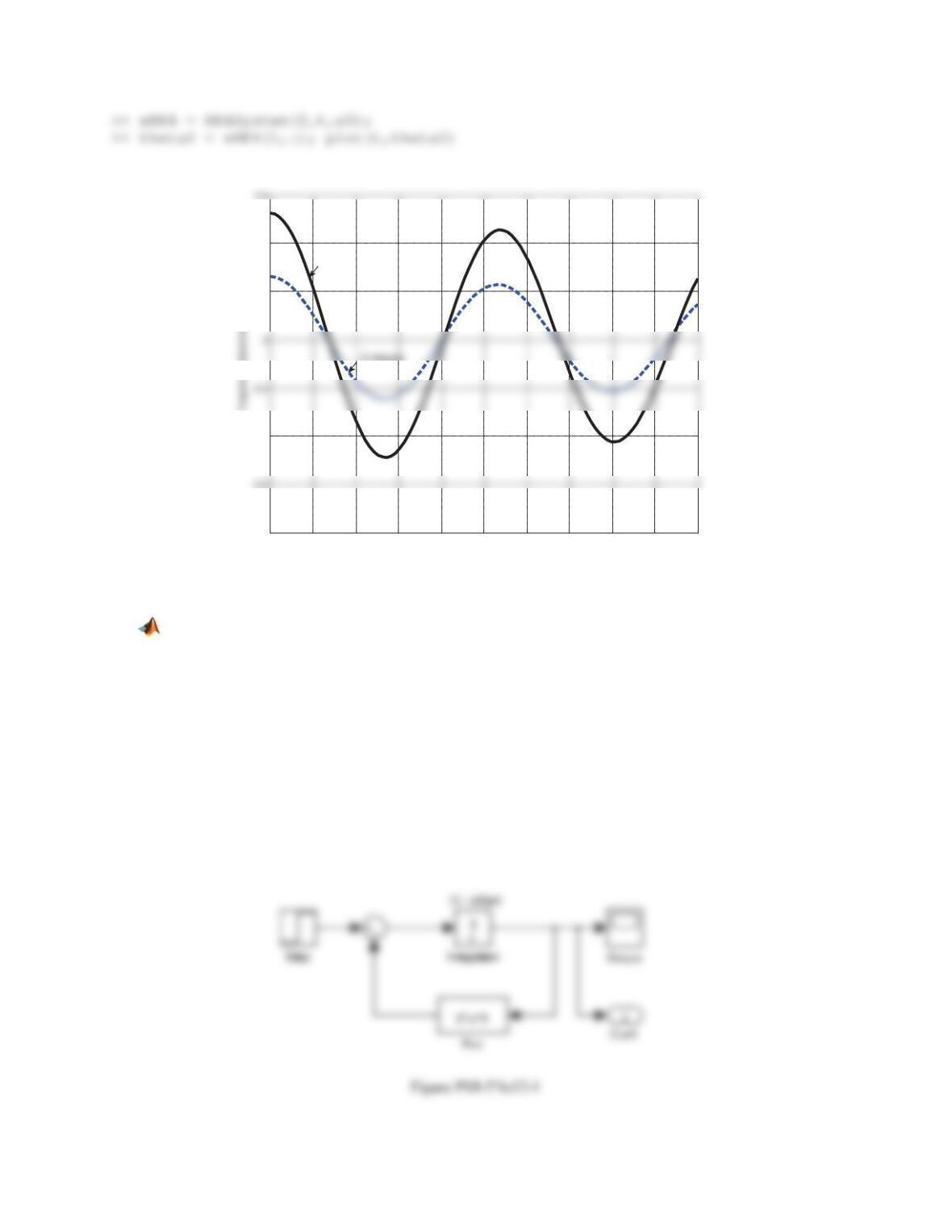
13. Consider
11
1112
2
2
212
(0) 1
21cos
, (0) 1
1
x
xxxax t
x
xxx
°
®
°
¯
where
a
is a parameter. Using RK4 solve the system for
1a
,
2a
, and plot the two resulting
1()xt
,
010tdd
, in the same graph.
Solution
>> t=linspace(0,10); x0=[1;1];
>> f1=inline(‘[-2*x(1,1)*abs(x(1,1))+x(2,1)-1+1/2*cos(t);-x(1,1)-x(2,1)-
377
Figure Review8No13
14. The nonlinear state-variable equations for a dynamic system are derived as
12 1
32
21 2
2 0.7sin (0) 1
, (0) 0
3 8
xx tx
x
xx x
°
®
°
¯
Plot 2()xt
,
010tdd
, by
(a) Using the RK4 method.
(b) Simulating the Simulink model of the system.
Solution
(a)
>> t=linspace(0,10); x0=[1;0];
0 1 2 3 4 5 6 7 8 9 10
-1
-0.8
-0.4
0
0.2
0.6
1
Time
x1 (a=2)
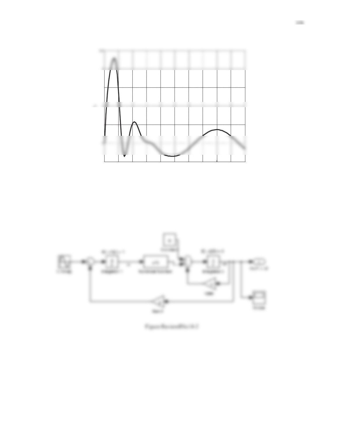
Figure Review8No14-1
(b) The Simulink model is built as shown in Figure Review8No14-2. Simulation will result in the exact same plot as
in (a).
0 1 2 3 4 5 6 7 8 9 10
-0.5
0.5
1.5
Time
x