399
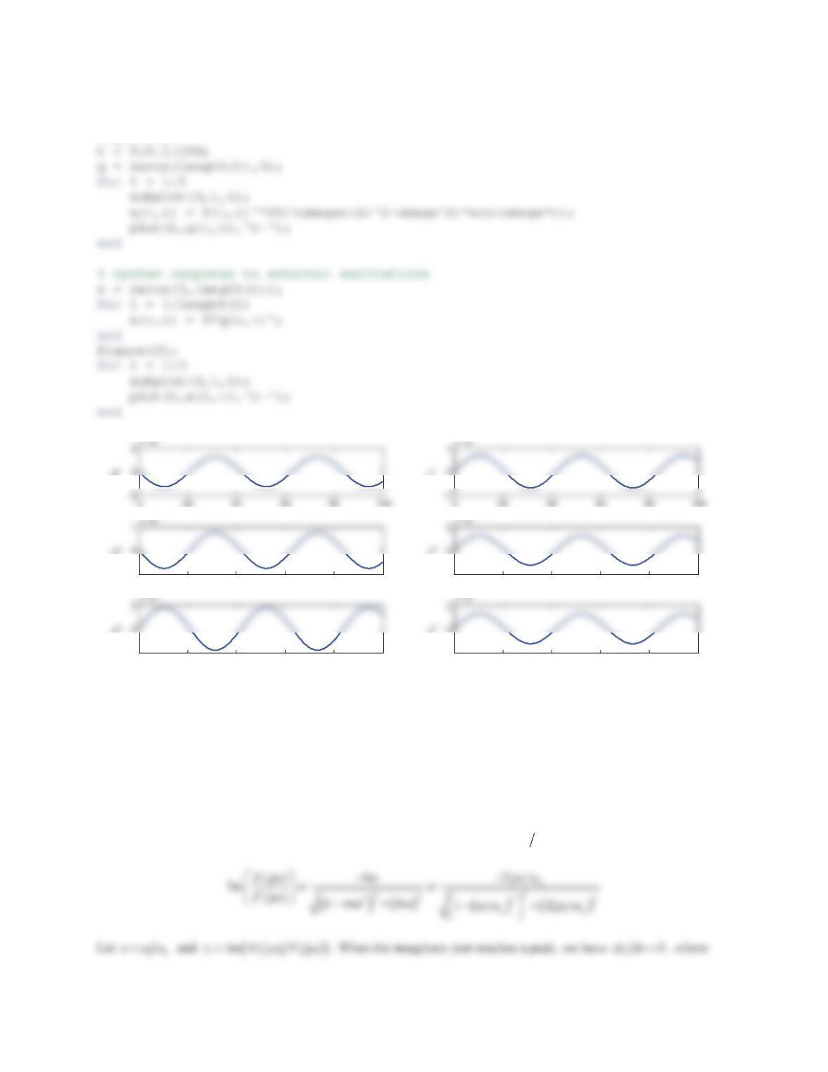
% modal response to external excitations
f0 = [0.15 0 0]’; omega = 0.15;
figure(1);
-5
q
020 40 60 80 100
-1
-5
q
020 40 60 80 100
-2
-6
Time (s)
q
-6
x
020 40 60 80 100
-5
-7
x
020 40 60 80 100
-2
-7
Time (s)
x
Figure PS9-4 No12a Modal responses. Figure PS9-4 No12b System responses.
Problem Set 9.5
1. For a single-degree-of-freedom system, denote the Fourier transforms of the displacement response and
excitation force as XMȦ DQG FMȦ, respectively. The expression of the imaginary part of the frequency
response function XMȦFMȦ LV JLYHQ E\ (TXDWLRQ 3URYH WKDW WKH LPDJLQDU\ SDUW UHDFKHV D SHDN DW
resonance.
Solution
The expression of the imaginary part of the frequency response function (jȦ MȦXF
is given by
400
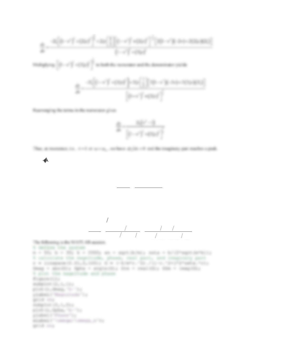
2. Accelerations are often measured in vibration testing. For a single-degree-of-freedom system, denote the
Fourier transforms of the acceleration response and excitation force as AMȦ DQG FMȦ, respectively. The
expression of the frequency response function AMȦFMȦLVJLYHQE\
2
2
(j ) .
(j ) j
A
Fkm b
ZZ
ZZ Z
Using MATLAB, write an m-file to plot the magnitude, phase, real part, and imaginary part of the frequency
response versus ȦȦn.Assume that m= 50 kg, b= 30 N·s/m, and k= 2000 N/m.
Solution
The frequency response function
(jȦ MȦAF
can be rewritten as
2
2
n
22
2
nn
1ȦȦ
(jȦ Ȧ
(jȦ Ȧ M Ȧ 1ȦȦ Mȗ ȦȦ
m
Ak
Fmkbk
0.05
0.1
0.15
00.5 11.5 2
0
1
3
Phase
0
00.5 11.5 2
0
0.05
0.1
0.2
Imaginary Part
3. Rods, beams, plates, and so on are continuous systems, which have an infinite number of degrees of freedom
and an infinite number of modes. For simplicity, assume that a cantilever beam is approximated as a single-
degree-of-freedom mass–damper–spring system, for which the natural frequency is close to the first mode of the
beam. The parameters of the cantilever beam are length L= 0.5 m, width b= 0.025 m, thickness h= 0.005 m,
GHQVLW\ȡ kg/m3, and Young’s modulus E= 210 × 109N/m2.
a. It is known that the equivalent mass for the beam is meq =m/3, where mis the actual mass of the beam.
Determine the equivalent stiffness keq for the beam. Calculate the natural frequency of the equivalent
single-degree-of-freedom system.
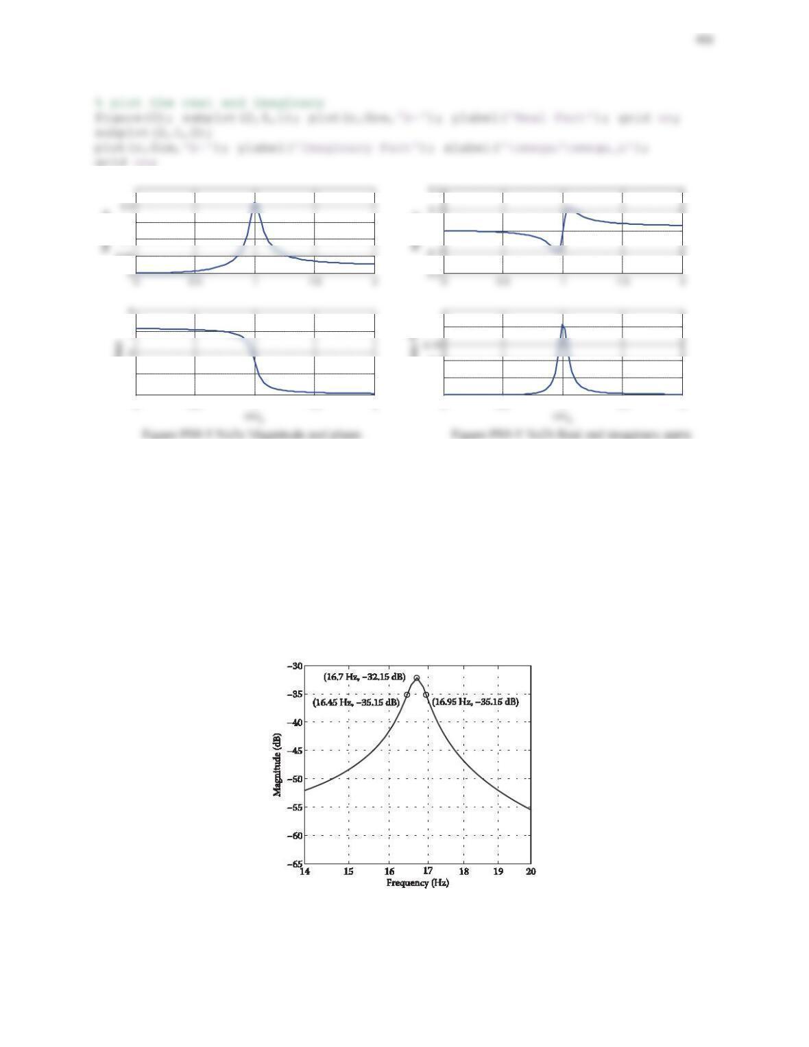
b. Figure 9.29 is the measured frequency response of the cantilever beam for the first mode. Determine the
natural frequency and the damping ratio based on the given information in the plot.
c. Compare the frequencies obtained in Parts (a) and (b). What is the error if the cantilever beam is
approximated as a single-degree-of-freedom system?
Figure 9.29 Problem 3.
Solution
a. Refer to Example 5.3. The equivalent stiffness for a cantilever beam is
eq 3
3
1312.5
44 0.5
Ebh
kL
N/m
b. From Figure 9.30, we have
16.7
n
f|
Hz and applying the method of half-power bandwidth gives
14.3 16.7 14.37%
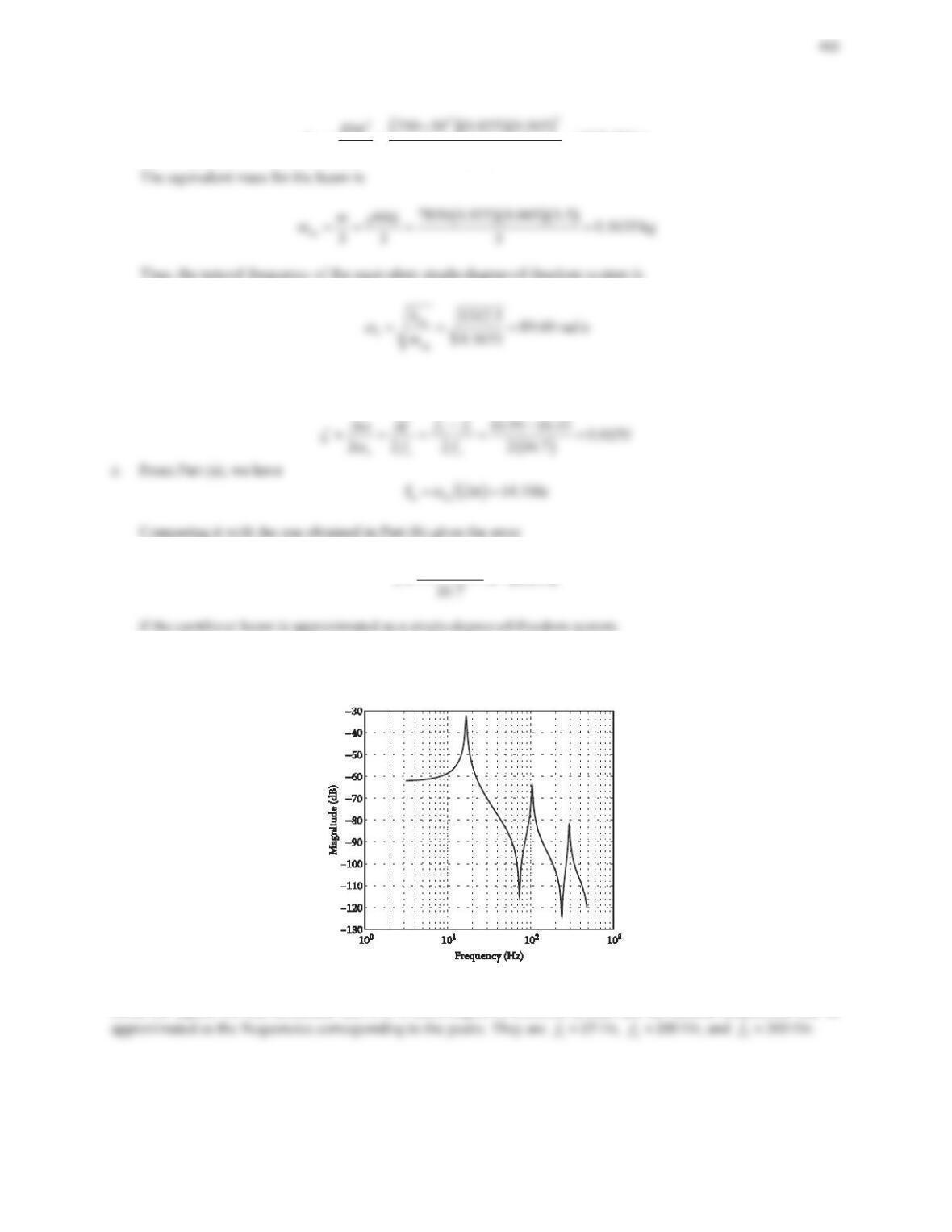
4. Figure 9.30 shows the magnitude of an experimentally determined frequency response. Estimate the degree-of-
freedom of the system and its natural frequencies.
Figure 9.30 Problem 4.
Solution
From the figure, we can determine that it is a three-degree-of-freedom system and the natural frequencies can be
Review Problems
1. Consider the single-degree-of-freedom system shown in Figure 5.42.
403
a. DetHUPLQHWKHXQGDPSHGQDWXUDOIUHTXHQF\Ȧn,WKHGDPSLQJUDWLRȗ,DQGWKHGDPSHGQDWXUDOIUHTXHQF\Ȧd.
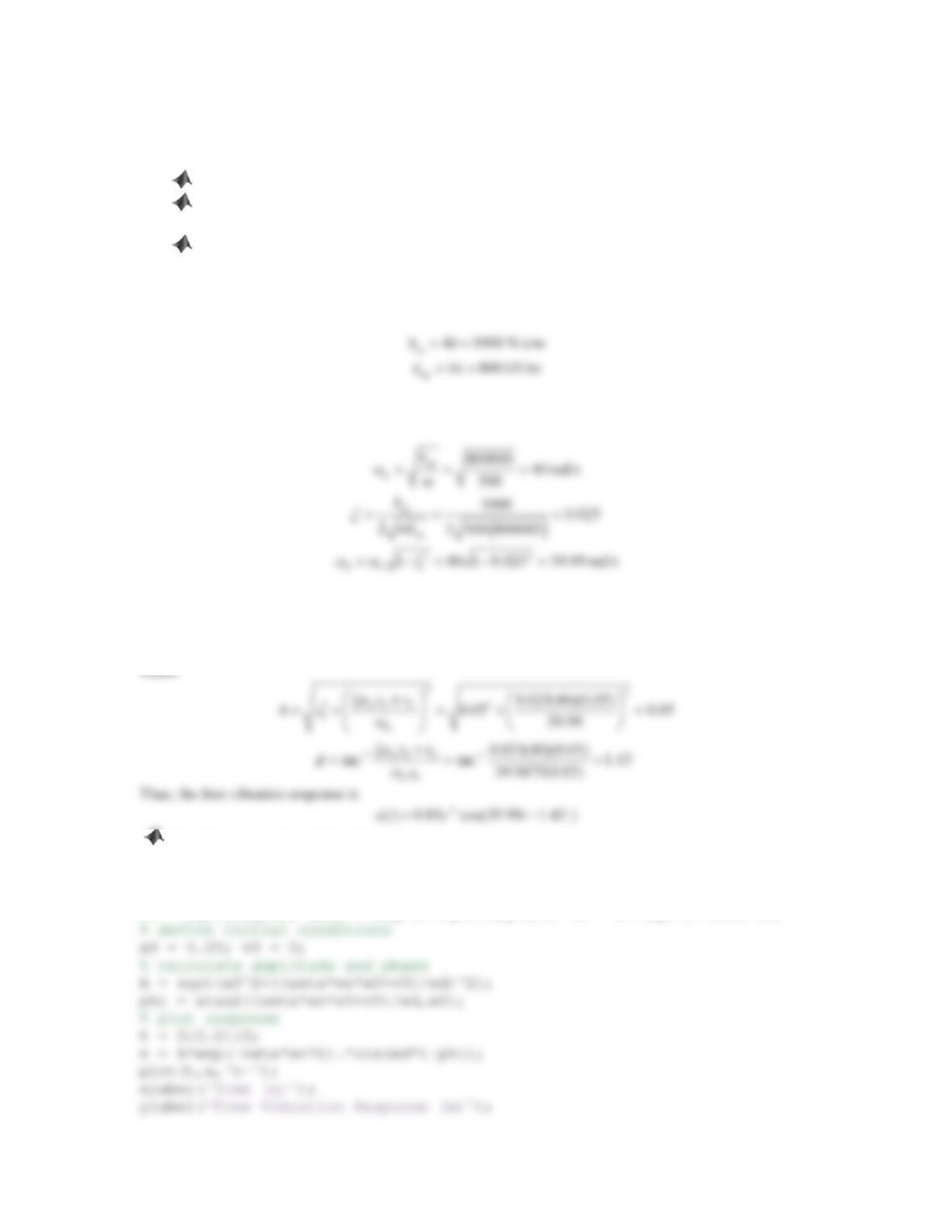
b. Assume f(t) = 0. Find the free vibration response of the system subjected to the initial conditions x(0) =
0.05 m and
(0) 0m/sx
.
c. Write a MATLAB m-file to plot the system’s response obtained in Part (b).
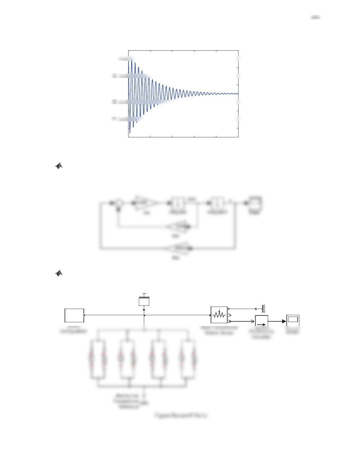
d. Construct a Simulink®block diagram based on the differential equation of motion of the system and
find the free vibration response.
e. Build a Simscape model of the physical system and find the free vibration response.
Solution
a. As shown in Figure 5.42, m= 500 kg. Four same spring-damping units are connected in parallel, where b= 250
Ns/m and k= 200 kN/m. Thus, the equivalent damping is
The differential equation of motion of the system is
eq eq
mx b x k x f
. We have
b. Assume
() 0ft
. The free vibration response of the system subjected to the initial conditions x(0) = 0.05 m
and
(0) 0m/sx
is
n
ȗȦ
d
() cos(Ȧ
t
xt Ae t
I
c. The following is the MATLAB session.
% define system parameters
m = 500; beq = 1000; keq = 800e3;
% calculate natural frequency, damping ratio, and damped natural frequency
wn = sqrt(keq/m); zeta = beq/(2*sqrt(keq*m)); wd = wn*sqrt(1-zeta^2);
0 1 2 3 4 5
-0.05
-0.04
-0.02
0
0.01
0.03
0.05
Time (s)
Figure Review9 No1a
d. The Simulink block diagram is shown in Plot (b). Set the initial velocity (by double-clicking the
Integrator block) to 0 and the initial displacement (by double-clicking the Integrator1 block) to
0.05. The response of the system is the same as the one shown in Plot (a).
Figure Review9 No1b
e. The Simscape block diagram is shown in Plot (c), which returns the same curve in Plot (a).
x
f(x)=0
PS S
Mechanical
Translational
Reference1
Mass
R
C
V
P
2. Consider the single-degree-of-freedom system shown in Figure 5.42.
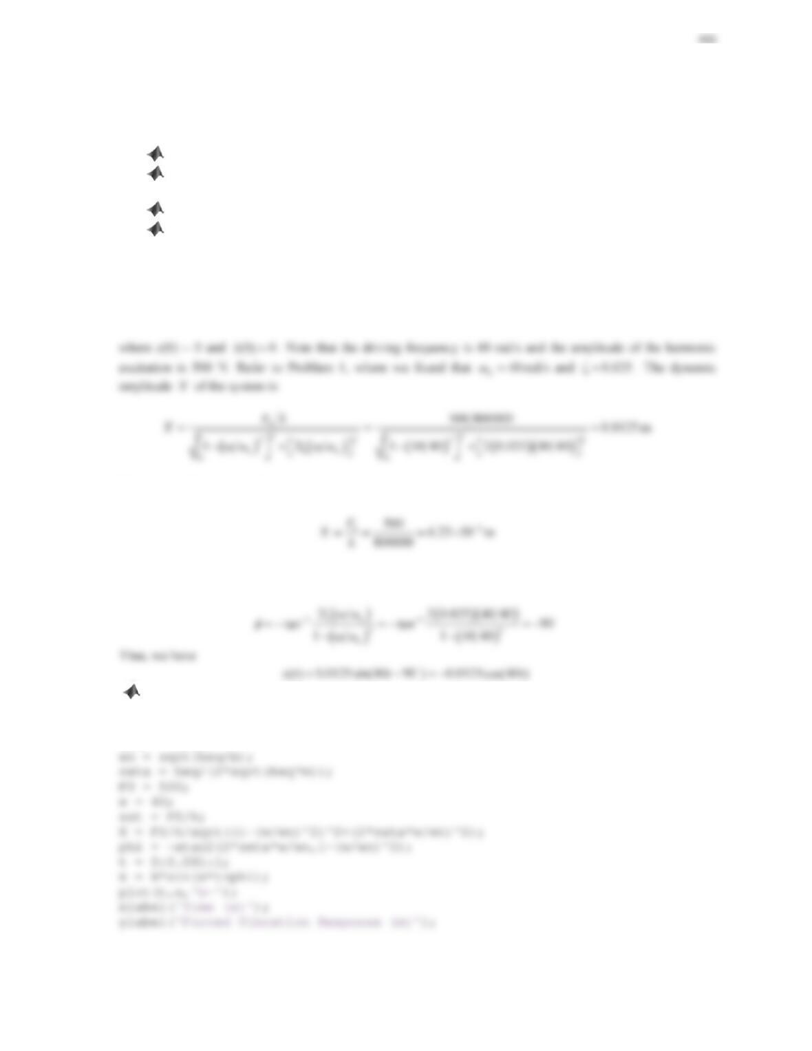
a. Assume f(t) = 500sin(40t) and initial conditions x(0) = 0 and (0) 0x
. Determine the dynamic amplitude X
and the static deflection xst of the system. Find the forced vibration response of the system.
b. Write a MATLAB m-file to plot the system’s response obtained in Part (a).
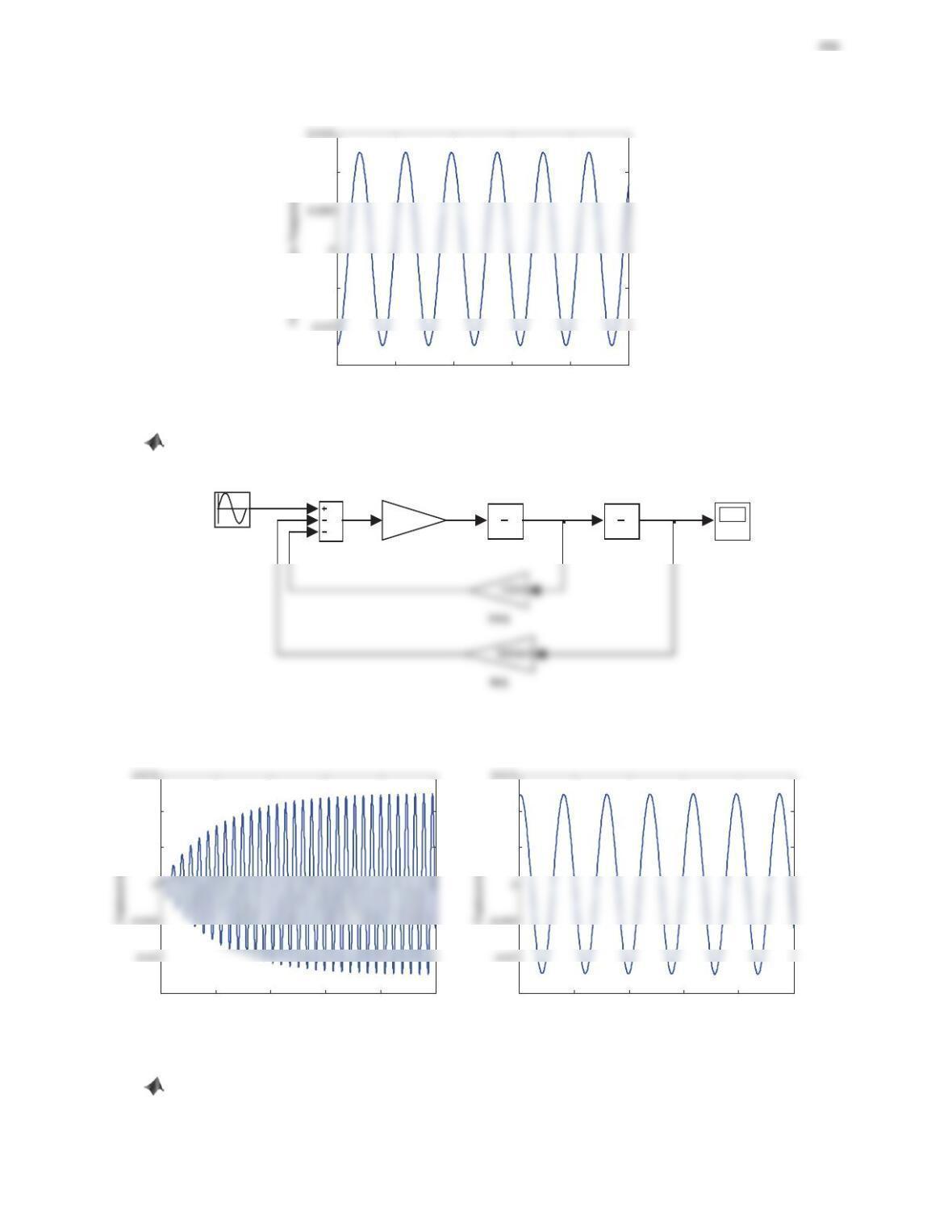
c. Construct a Simulink®block diagram based on the differential equation of motion of the system and
find the forced vibration response.
d. Build a Simscape model of the physical system and find the forced vibration response.
e. Assume that the driving frequency varies from 0 to 100 rad/s. Write a MATLAB m–file to plot the
dimensionless ratio X/xst YHUVXVWKHGULYLQJIUHTXHQF\Ȧ
Solution
a. Refer to Part (a) in Review Problem 1. The differential equation of motion of the system is
500 1000 800000 500sin(40 )xx x t
The static deflection st
xof the system is
The steady-state response of the system is
() sin Ȧxt X t
I
where
0.0125X
m and
b. The following is the MATLAB session.
m = 500;
beq = 1000;
keq = 800e3;
00.2 0.4 0.6 0.8 1
-0.015
-0.005
0.01
Time (s)
Figure Review9 No2a
c. The Simulink block diagram is shown in Plot (b) and the response of the system is shown in Plot (c). Note
this is the total response of the system, and the steady-state response is the same as the one shown in Plot (a).
xdot x
Sine Wave
Scope
1
s
Integrator1
1
s
Integrator
1/500
1/m
Figure Review9 No2b
0 1 2 3 4 5
-0.015
0.005
0.01
Time (s)
44.2 4.4 4.6 4.8 5
-0.015
0.005
0.01
Time (s)
Figure Review9 No2c
d. The Simscape block diagram is shown in Plot (d), which returns the same response shown in Plot (c).

407
f(x)=0
Converter Scope
Converter
Mechanical
Mechanical
Motion Sensor
e. The following is the MATLAB session.
w = linspace(0,100,500);
r = w./wn;
Xxst = 1./sqrt((1-r.^2).^2+(2*zeta.*r).^2);
020 40 60 80 100
0
4
6
12
14
16
18
20
Z (rad/s)
Figure Review9 No2d
3. A machine can be considered as a rigid mass with a rotating unbalanced mass. To reduce the vibration, the
machine is mounted on a support system with a stiffness of 10 kN/m. Assume that the total mass M= 10 kg and
the unbalanced mass m= 0.5 kg. Determine the range of the damping ratio of the support system so that the
vibration amplitude will not exceed 10% of the rotating mass’s eccentricity when the machine operates at a
speed of 350 rpm.
408
Solution
For a system with rotating unbalance, the dimensionless ratio
The vibration amplitude will not exceed 10% of the rotating mass’s eccentricity, i.e.,
where M = 10 kg, m= 0.5 kg, k= 10 kN/m, and Z= 350 rpm = 36.65 rad/s. The natural frequency of the system is
n
Ȧ kM
rad/s. The above inequality can be rewritten as
4. As shown in Figure 9.31, a machine of a mass M= 150 kg is mounted on a fixed-fixed steel beam with
negligible mass. The parameters of the beam are given as follows: Young’s modulus of the beam E= 210 GPa,
width b= 0.75 m, and thickness h= 3 cm. The rotating unbalance in the machine is me = 0.015 kgm. The
machine runs at a speed of 2400 rpm and the maximum allowable displacement is 4 mm. Determine the length
of the beam. Assume damping to be negligible.
Figure 9.31 Problem 4.
Solution
The system shown in Figure 9.31 can be simplified as a single-degree-of-freedom mass-spring system with rotating
unbalance. Neglect the damping. The maximum allowable displacement of the machine is 4 mm, i.e.,
Solving for the frequency ratio ȦȦngives
409
The machine runs at a speed of 2400 rpm. Thus, the natural frequency of the machine should be
Pick Ȧn= 255 rad/s. Then, the equivalent spring stiffness of the system is
2
eq n
ȦkM
. Note the equivalent spring
stiffness for a fixed-fixed beam is
33
eq
16k Ebh L
. Solving for the length gives
5. A 110-kg machine is placed on a floor that vibrates with a frequency of 20 Hz. The maximum acceleration of
the floor is 15 cm/s2. A vibration isolator consisting of four parallel-connected springs is designed to protect the
machine from the vibration of the floor. Assume that the damping ratio of the isolator is 0.1 and the maximum
allowable acceleration is 2.25 cm/s2. Determine the stiffness of each spring.
Solution
The maximum allowable accelerations of the machine and the floor are 2.25 cm/s2and 15 cm/s2, respectively. Thus,
the displacement transmissibility is
22
22
00
Ȧ 0.15
Ȧ
XX
ZZ
u
u
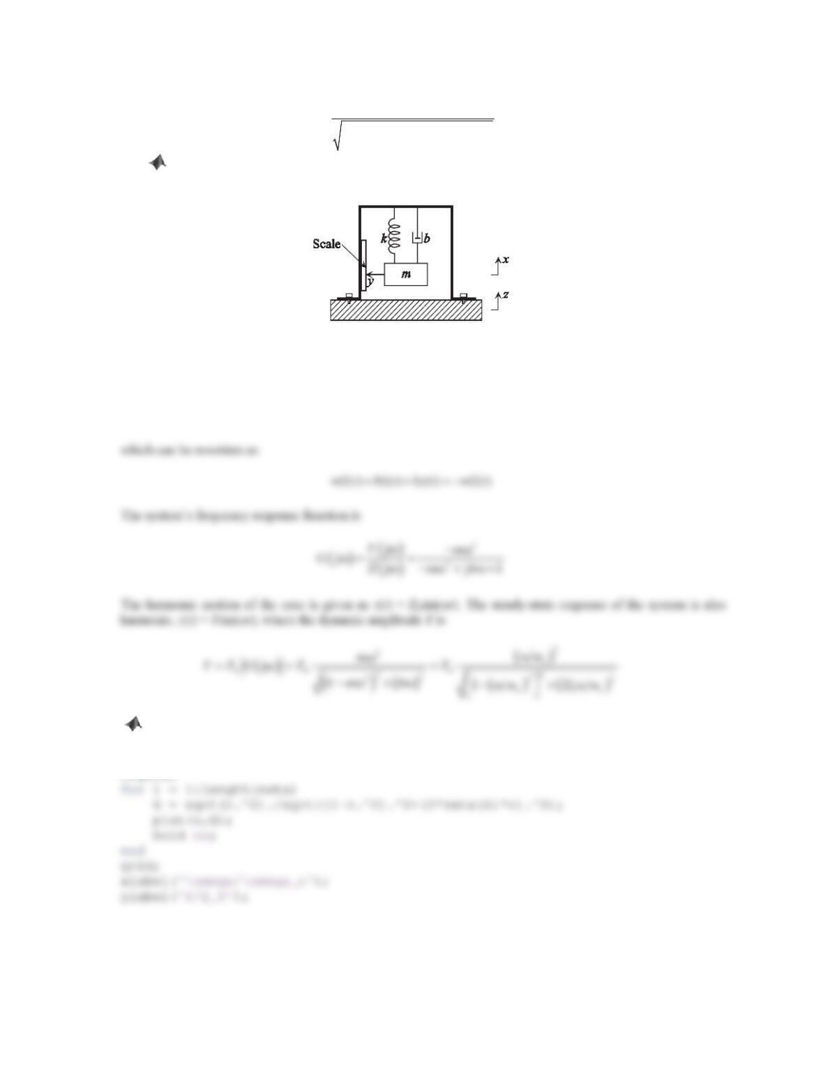
6. Many vibration measuring instruments consist of a case containing a mass–damper–spring system, as shown in
Figure 9.32. The displacement of the mass relative to the case is measured electrically. Denote the displacement
of the mass, the displacement of the case, and the displacement of the mass relative to the case as x(t), z(t), and
y(t), respectively, where y(t) = x(t)íz(t). Assume harmonic excitation, z(t) = Z0sin(Ȧt).
a. Show that the amplitude Yis given by
410
2
n0
22
2
nn
(/ ) .
1(/ ) 2 /
YZ
ZZ
ªº
ZZ ]ZZ
¬¼
b. Using MATLAB®, write an m-file to plot the frequency response Y/Z0YHUVXVȦ/Ȧnfor different values
RIGDPSLQJUDWLRȗ , 0.25, 0.5, 0.7, and 1.0.
Figure 9.32 Problem 6.
Solution
a. For the mass-damper-spring system, the differential equation of motion is
() () () () ()mx t bx t kx t bz t kz t
>@>@>@
() () () () () () ()mxtzt bxtzt kxtzt mzt
b. The following is the MATLAB session.
zeta = [0.1 0.25 0.5 0.7 1.0];
r = 0:0.01:2.5;
figure;
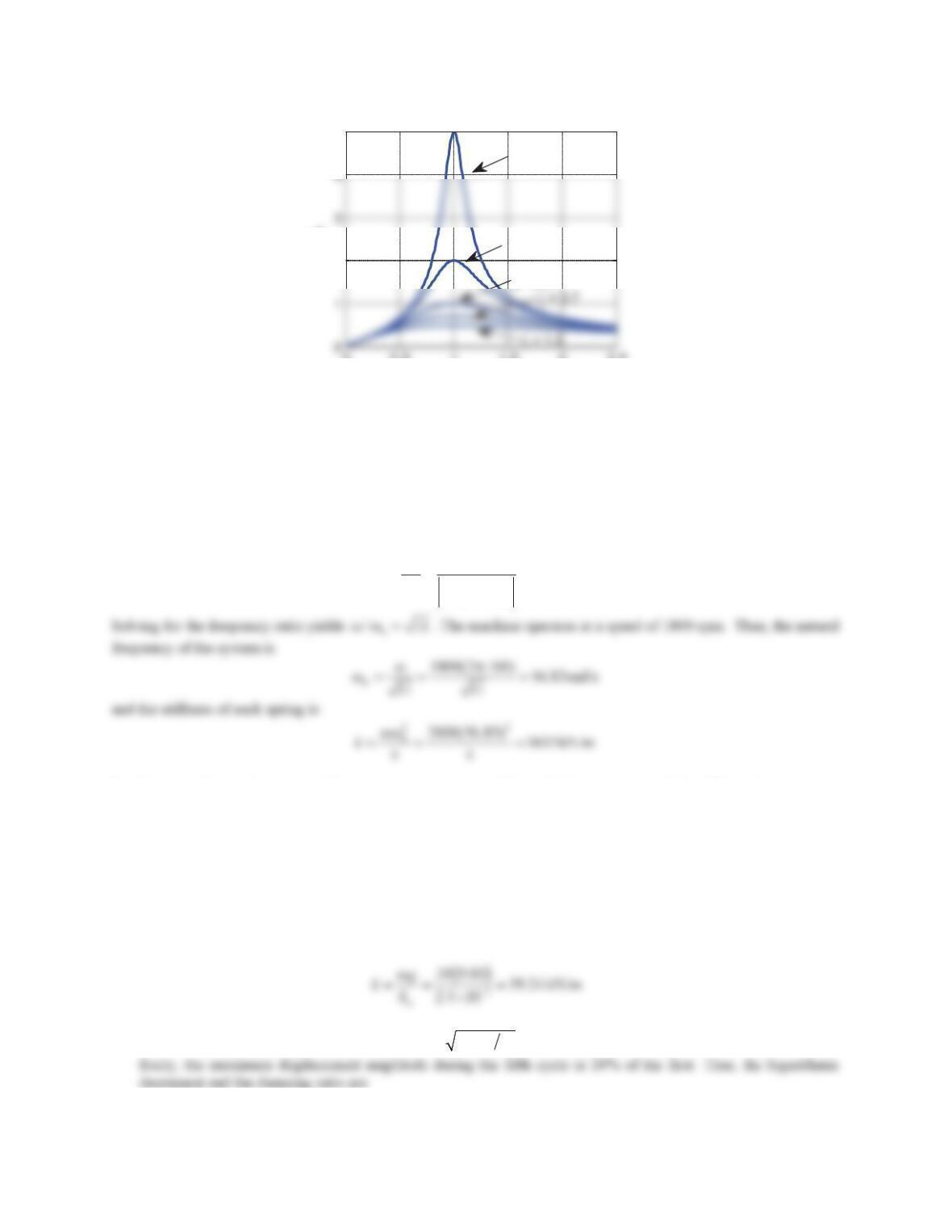
411
00.5 11.5 22.5
2
5
Z/Z
n
Y/Z
0
] = 0.1
] = 0.25
] = 0.5
Figure Review9 No6
7. A 2000-kg rotating machine is mounted on a vibration isolator consisting of four parallel-connected springs.
The machine operates at a speed of 1800 rpm. Determine the stiffness of each spring so that the force
transmitted to the ground is reduced by 90%. Assume that all the springs are identical and damping is
negligible.
Solution
The force transmitted to the ground is reduced by 90%. This implies that FT/F0= 0.1. Neglecting the damping, we
have
T
2
0n
10.1
1/
F
F
ZZ
8. Consider the single-degree-of-freedom system shown in Figure 9.15a, where m= 10 kg. When the mass is in
equilibrium, the static deformation of the spring is 2.5 mm. When the mass is allowed to vibrate freely, the
maximum displacement amplitude during the fifth cycle is 20% of the first. Assume that a harmonic excitation
force is applied to the system.
a. Determine the minimum allowable driving frequency if the force transmitted to the ground is less than the
excitation force.
b. If the allowable force transmissibility is 20%, determine the stiffness of the spring.
Solution
a. The static deformation of the spring is 2.5 mm. Thus, the stiffness of the spring is
and the natural frequency of the system is
n
Ȧ
rad/s. When the mass is allowed to vibrate
412
If the force transmitted to the ground is less than the excitation force, we have
Thus, the frequency ratio
n
ȦȦ
is greater than
2
. This result can also be obtained by observing the
transmissibility plot in Figure 9.12. The minimum allowable driving frequency is
which is equivalent to
42
nn
Ȧ Ȧ Ȧ Ȧ
9. Consider the vibration absorber shown in Figure 9.16. It is known that two new resonant frequencies in the
neighborhood RIWKHH[FLWDWLRQIUHTXHQF\DUHFUHDWHG‘HQRWH WKHWZRQHZQDWXUDO IUHTXHQFLHVDV Ȧn1 DQGȦn2.
$VVXPHȞ ’HWHUPLQHȦn1/Ȧ1DQGȦn2/Ȧ1IRUWKHIROORZLQJFDVHVȝ DQG25.
Solution
For the vibration absorber in Figure 9.16, the equation of motion is
111221
1
22 2 2 2
0sin(Ȧ
00
mxkkkx
Ft
mx k k x
½ ½
ªºª º½
®¾ ®¾®¾
«»« »
¯¿
¯¿ ¯¿
¬¼¬ ¼
413
which has two roots of
2
1
ȦȦ
, corresponding to
2
n1 1
ȦȦ
and
2
n2 1
ȦȦ
. The results for the different values of
ȝare listed below.
Table Review9 No9
ȝ0.05 0.1 0.15 0.2 0.5
10. A 75–kg table saw is driven by a motor, which runs at a constant speed of 180 rpm and produces a 13-N force.
Assume that the stiffness provided by the table legs is 2500 N/m and the damping is negligible.
a. Determine the dynamic amplitude of the table.
b. Design a vibration absorber to reduce the table oscillation to zero. Assume that the maximum allowable
displacement of the absorber is 2 mm. What iVWKHYDOXHRIWKHPDVVUDWLRȝ?
Solution
a. The natural frequency of the table saw is
1
2500 =5.77 rad/s
75
Z
b. The natural frequency of the absorber is required to be the same as the excitation frequency,
The maximum allowable displacement amplitude of the absorber is 2 mm. Considering the magnitude only, the
spring stiffness of the absorber can be obtained as
11. Consider the linearized model of the double pendulum system in Example 5.15. Assume m= 1 kg and L = 1 m.
a. Use the modal analysis approacKWRGHWHUPLQHWKHUHVSRQVHRIWKHV\VWHPWRWKHLQLWLDOH[FLWDWLRQVș1(0) =
0.05 rad, ș2(0) = 0.1 rad,
1(0) 0 rad/sT
, and
2
(0) 0 rad/sT
.
b. Write a MATLAB m-file and plot the response of the system.
c. Construct a Simulink®block diagram based on the linearized model and find the response of the
system.
414
Solution
a. Refer to Example 5.15. The linearized model of the double pendulum system is
where m= 1 kg and L = 1 m. Solving the eigenvalue problem
gives the natural frequencies
1
Ȧ
rad/s,
2
Ȧ
rad/s
For ș1(0) = 0.05 rad, ș2(0) = 0.1 rad,
1
(0) 0 rad/sT
, and
2
(0) 0 rad/sT
, the modal responses are
1
() (0)cos(Ȧ VLQȦ
Ȧ
TT
rr r r r
r
qt t t r XMș;0ș
The response of the system to the given initial excitations is
b. Refer to Problem 9 in Problem Set 9.4. The mass matrix, stiffness matrix, and initial conditions are set as
follows.
m = 1;
L = 1;
g = 9.81;
M = [2*m*L^2 m*L^2; m*L^2 m*L^2]; % mass matrix
-0.1
0.1
0.2
0 2 4 6 8 10
-0.02
0.01
Time (s)
-0.05
0.1
0246810
-0.1
0.05
Time (s)
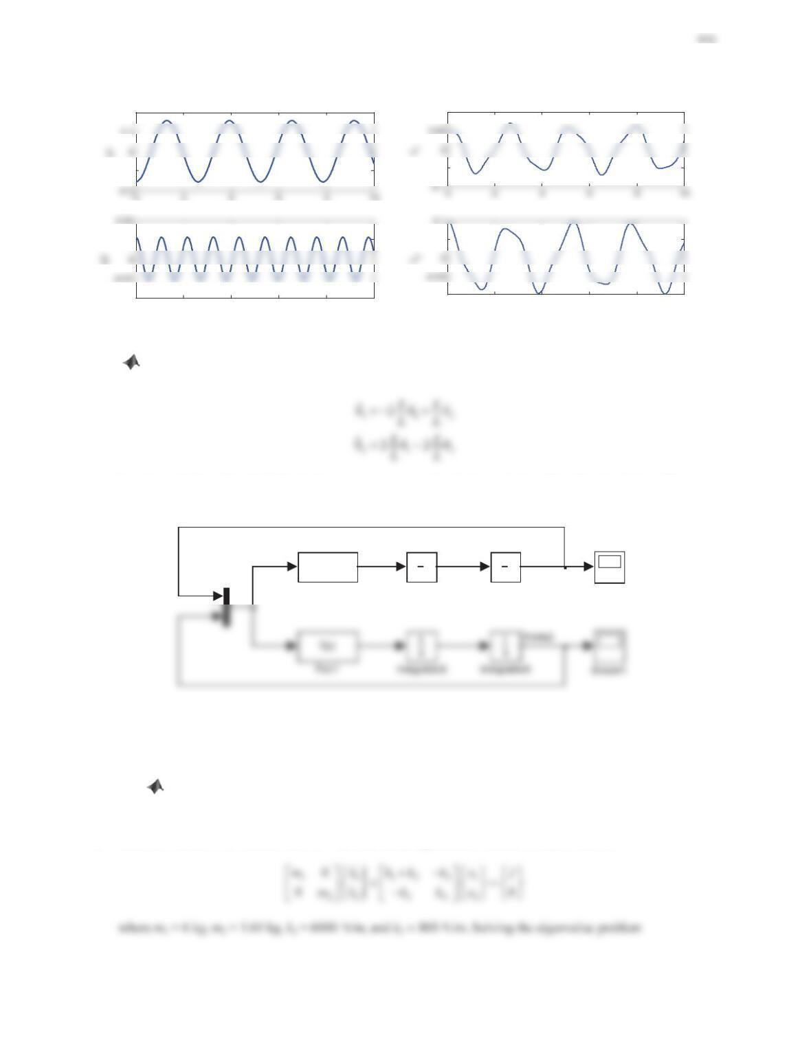
Figure Review9 No11a Modal responses. Figure Review9 No11b System responses.
c. Solving for the accelerations
1
ș
and 2
ș
using the linearized model of the system gives
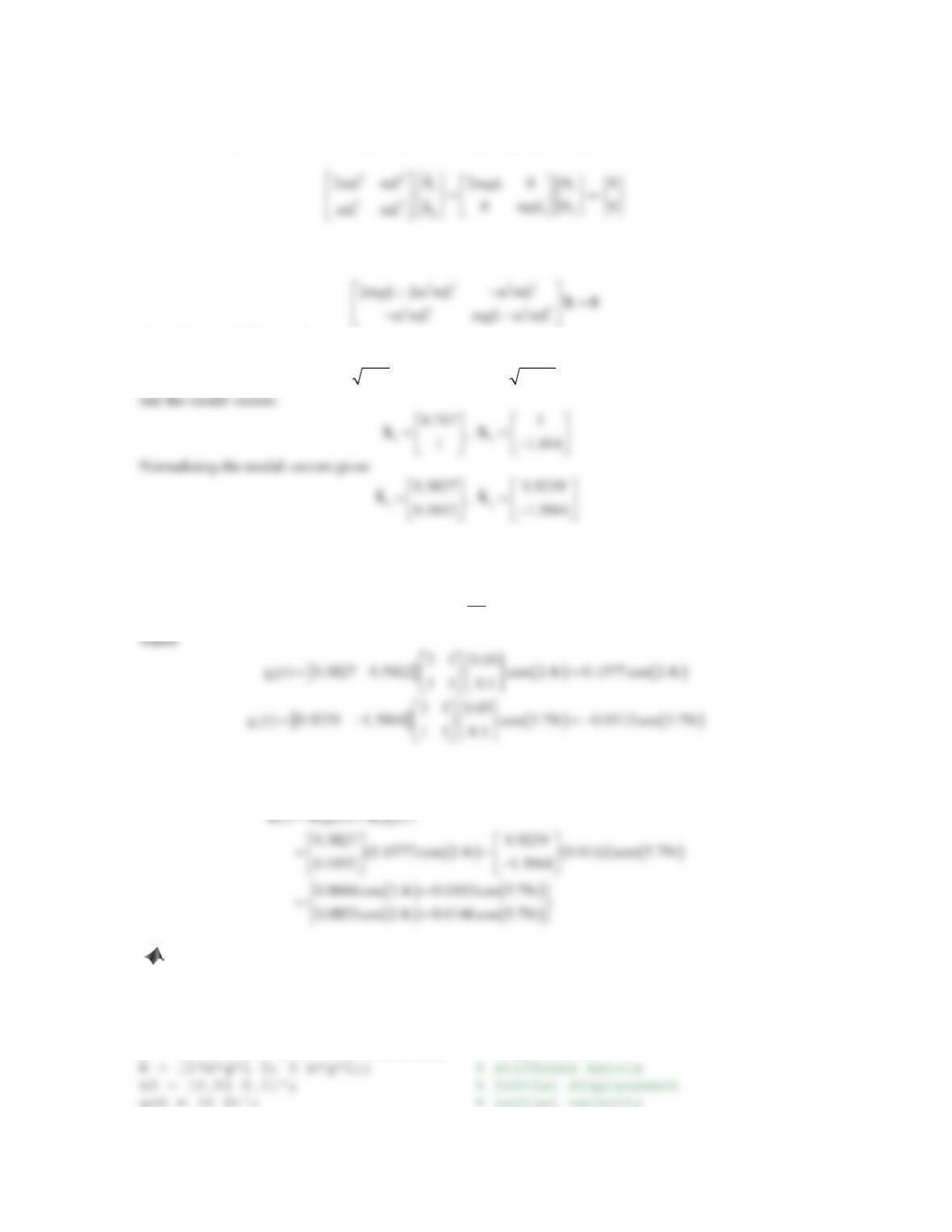
based on which a Simulink block diagram is constructed and shown below. Run the simulation. The same
responses as in Figure Review9 No11b can be obtained.
theta1
Scope
1
s
Integrator1
1
s
Integrator
f(u)
Fcn
Figure Review9 No11c Simulink block diagram.
12. Consider the two-degree-of-freedom mass–spring system in Figure 5.118 (Problem 3 in Problem Set 5.6).
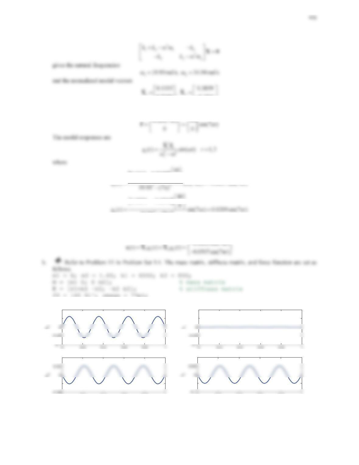
a. Use modal analysis to determine the response of the system to the harmonic excitation f= 40sin(7St) N.
b. Write a MATLAB m-file, plot the response of the system, and compare the result with those obtained
with Simulink and Simscape simulations.
Solution
a. Refer to Problem 3 in Problem Set 5.6. The differential equations of motion in matrix form is
0.7359
¬¼
0.2541
¬¼
The force vector can be written as
>@
0.1333 0.7359 0
®¾
¯¿
>@
0.3859 0.2541 0
34.94 (7ʌ
®¾
The response of the system to the given harmonic excitation is
0.05
0.1
00.2 0.4 0.6 0.8 1
-0.02
0.04
Time (s)
0.05
0.1
00.2 0.4 0.6 0.8 1
-0.05
0.1
Time (s)
Figure Review9 No12a Modal responses. Figure Review9 No12b System responses.
417
c. Solving for the accelerations
1
x
and 2
x
gives
>@
1112
22
1()xfkkxx
mk
based on which a Simulink block diagram is constructed and shown below. Run the simulation. The same
responses as in Figure Review9 No12b can be obtained.
x1
Scope
1
s
Integrator1
1
s
Integrator
f(u)
Fcn
Figure Review9 No12c Simulink block diagram.
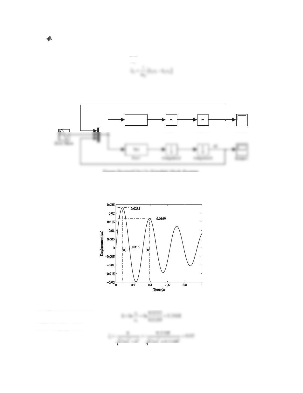
13. A single-degree-of-freedom system undergoes free vibration. Figure 9.33 is the recorded displacement response
of the first three cycles. The mass of the system is known to be 1750 kg. Determine the stiffness kand the
damping bof the system.
Figure 9.33 Problem 13.
Solution
The logarithmic decrement is
and the damping ratio is
418
The damped natural frequency is
d
d
2ʌʌ
Ȧ
0.315T
rad/s and the undamped natural frequency is
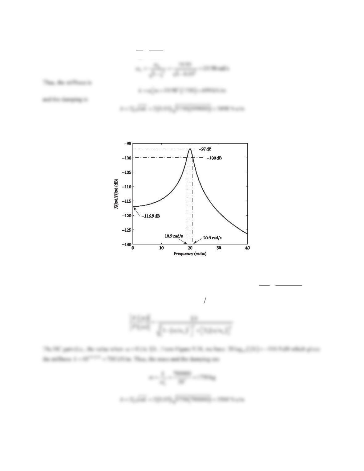
14. The frequency response of a single-degree-of-freedom system is shown in Figure 9.34. Determine the system’s
parameters including the mass m, the stiffness k, and the damping b.
Figure 9.34 Problem 14.
Solution
For small damping, the natural frequency can be estimated using the peak of the frequency response, i.e.,
n
Ȧ|
rad/s. Applying the half-power bandwidth method gives the damping ratio
n
Ȧ
ȗ
2Ȧ
‘
|
.
Note that the magnitude of the frequency response function
jȦMȦXF
is