Unlock document.
This document is partially blurred.
Unlock all pages and 1 million more documents.
Get Access
351
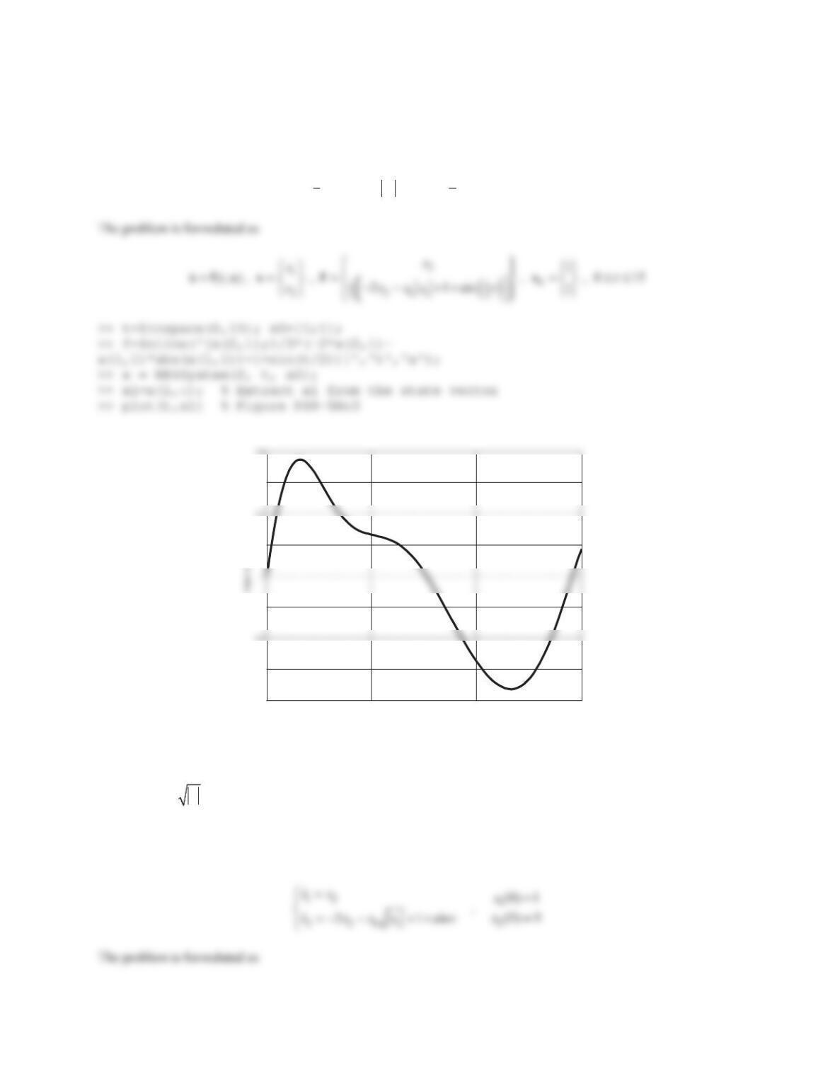
In Problems 5 through 10 determine the state vector via the formal-solution approach.
5.
21 1 0
, unit-step function , (0)
42 2 1
uu
ªºªº ½
®¾
«»«»
¬¼¬¼ ¯¿
xx x
Solution
>> A=[2 -1;-4 2]; B=[1;2]; x0=[0;1]; syms t tau
6.
24 2 1
, sin , (0)
12 1 0
uu t
ªºªº ½
®¾
«»«»
¬¼¬¼ ¯¿
xx x
Solution
>> A=[2 -4;-1 2]; B=[2;-1]; x0=[1;0]; syms t tau
7.
01 0 0
, , (0)
23 1 1
t
uue
ªºªº ½
®¾
«»«»
¬¼¬¼ ¯¿
xx x
Solution
>> A=[0 1;-2 -3]; B=[0;1]; x0=[0;-1]; syms t tau
352
8.
100 00 0
1
0 1 0 1 0 , , (0) 0
232 01 1
t
e
ªºªº ½
½
°° °°
«»«»
®¾ ®¾
«»«»°° °°
¯¿
«»«»
¬¼¬¼ ¯¿
xxuux
Solution
>> A=[1 0 0;0 -1 0;2 3 2]; B=[0 0;1 0;0 1]; x0=[0;0;1]; syms t tau
9.
100 0 0
0 1 0 0 , unit-step function , (0) 1
24 1 2 0
uu
ªºªº ½
°°
«»«»
®¾
«»«» °°
«»«»
¬¼¬¼ ¯¿
xx x
Solution
>> A=[1 0 0;0 1 0;-2 4 -1]; B=[0;0;2]; x0=[0;1;0]; syms t tau
10.
01 0 1
, unit-ramp function , (0)
02 1 0
uu
ªºªº ½
®¾
«»«»
¬¼¬¼ ¯¿
xx x
Solution
>> A=[0 1;0 -2]; B=[0;1]; x0=[1;0]; syms t tau
In Problems 11 and 12, the state-space representation of a system model is provided. Using the formal-solution
approach, find the response
()yt
.
11.
>@
0
01 1 1
, , , 1 1 , sin ,
4 4 2 1
uut
y
ªºªº ½
®®¾
«»«»
¯¬¼¬¼ ¯¿
xAxB
ABC x
Cx
Solution
>> A=[0 1;-4 -4]; B=[1;-2]; C=[1 1]; x0=[1;-1]; syms t tau
>> x=expm(A*t)*x0+int(expm(A*(t-tau))*B*sin(tau),tau,0,t);
353
12.
>@
0
102 00 1
1
, 0 1 1 , 1 0 , 1 0 1 , , 0
003 01 1
t
ye
ªºªº ½
½
°° °°
«»«»
®®¾®¾
«»«»
°°
¯°°
¯¿
«»«»
¬¼¬¼ ¯¿
xAxBu
ABCux
Cx
Solution
>> A=[1 0 2;0 -1 1;0 0 3]; B=[0 0;1 0;0 1]; C=[1 0 1]; x0=[1;0;1];
syms t tau
Problem Set 8.5
In Problems 1 through 6 find and plot the specified output using the RK4 method.
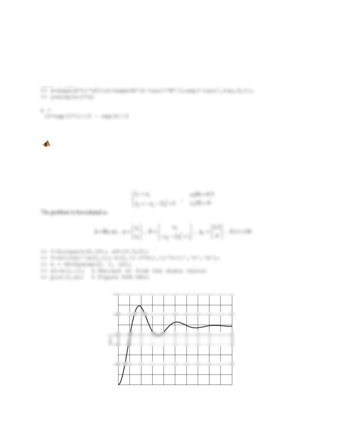
1.
3
2 1 , (0) 0.5 , (0) 0 , 0 10xx x x x t dd
Output:
()xt
Solution
With state variables
1
xx
and
2
xx
, the nonlinear state-variable equations are obtained as
Figure PS8-5No1
0 1 2 3 4 5 6 7 8 9 10
0.5
0.55
0.65
0.8
0.9
Time
354
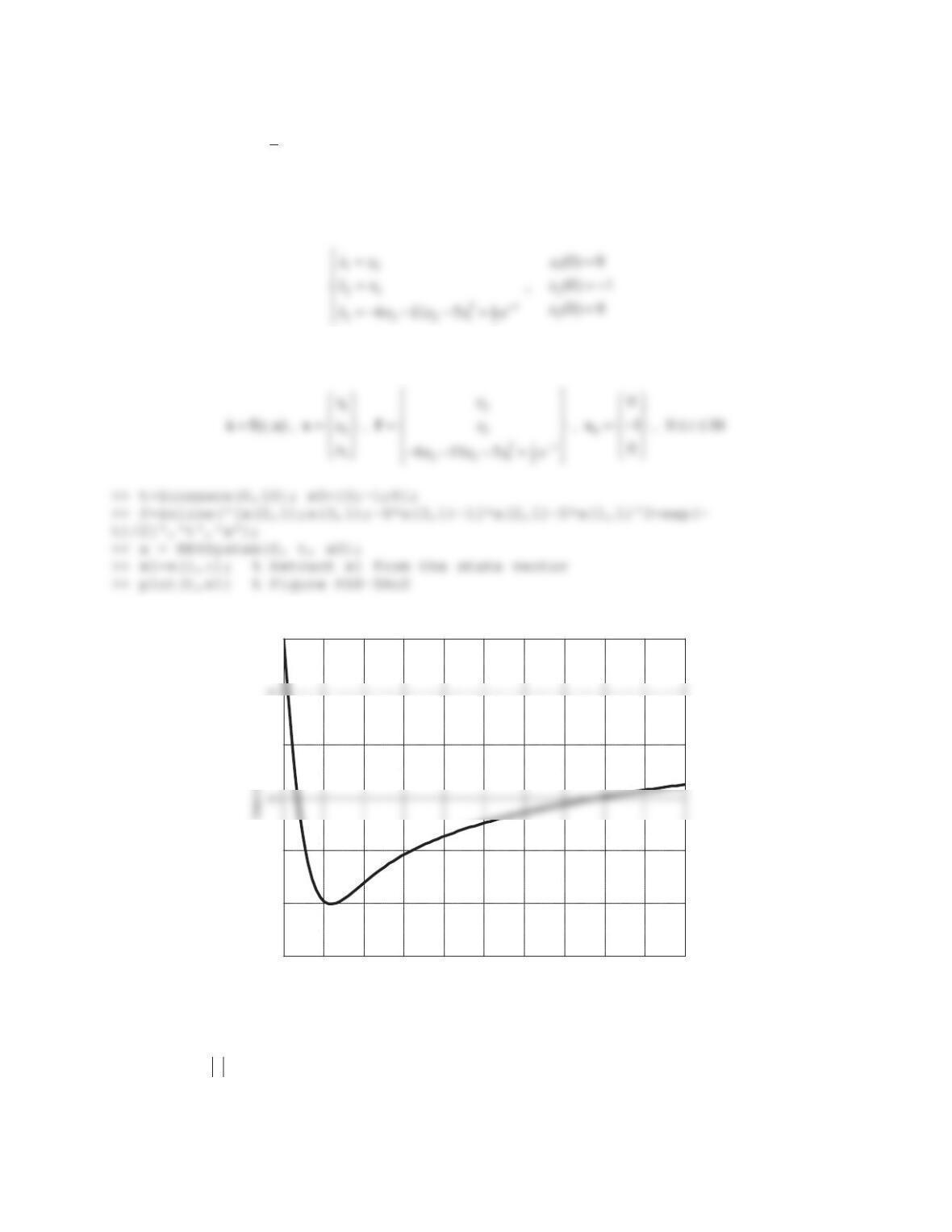
2.31
2
6 11 5 , (0) 0 , (0) 1 , (0) 0 , 0 10
t
xx xx e x x x t
dd
Output:
()xt
Solution
Choosing state variables
1
xx
,
2
xx
, and
3
xx
, the nonlinear state-variable equations are obtained as
The problem is formulated as
Figure PS8-5No2
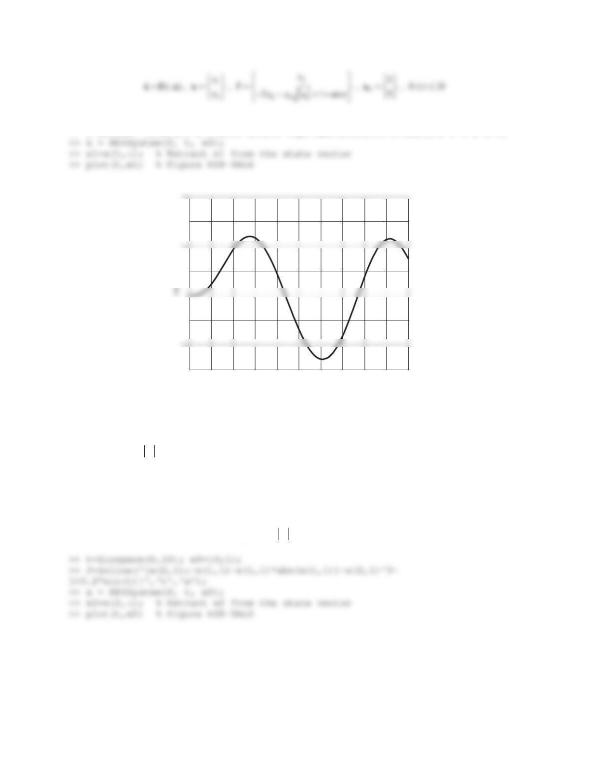
3.
3 2 1 sin( / 2) , (0) 1 , (0) 1 , 0 15
xxxx t x x t dd
Output:
()xt
0 1 2 3 4 5 6 7 8 9 10
-0.5
-0.4
-0.2
0
Time
355
Solution
With state variables
1
xx
and
2
xx
, the nonlinear state-variable equations are obtained as
12 1
11
2211 2
32
(0) 1
,
21sin (0) 1
xx x
xxxx t
x
°
®ªº
°¬¼
¯
Figure PS8-5No3
4.
2 1 sin , (0) 1 , (0) 0 , 0 10xxxx t x x t dd
Output:
()xt
Solution
With state variables
1
xx
and
2
xx
, the nonlinear state-variable equations are obtained as
0 5 10 15
0.2
0.4
0.8
1.2
1.6
Time
356
>> t=linspace(0,10); x0=[1;0];
>> f=inline('[x(2,1);-2*x(2,1)-x(1,1)*sqrt(abs(x(1,1)))+1+sin(t)]','t','x');
Figure PS8-5No4
5.
12 1
3
2
21112
(0) 0
, , 0 10
(0) 1
1 0.2sin
xx xt
x
xxxxx t
°dd
®
°
¯
Output: 2()xt
Solution
The problem is formulated as
2
1
0
3
2111 2
0
( , ) , , , , 0 10
1
1 0.2sin
x
x
tt
xxxx x t
½
½ ½
°°
dd
®¾ ® ¾ ®¾
¯¿
¯¿ °°
¯¿
xf x x f x
01 2 3 4 5 6 7 8 910
0.4
0.8
1.2
1.6
Time
357
Figure PS8-5No5
6.
31
112
2
21
(0) 0
2 , , 0 5
(0) 1
8sin
x
xxx t
x
xx t
°dd
®
°
¯
Output: 2()xt
Solution
The problem is formulated as
3
112
0
21
0
2
( , ) , , , , 0 5
1
8sin
xxx
tt
xxt
½
½ ½
°°
dd
®¾ ® ¾ ®¾
°°
¯¿
¯¿ ¯¿
xf x x f x
0 1 2 3 4 5 6 7 8 9 10
-0.8
-0.4
0.2
0.4
0.8
1
Time
-1
0
0.5
1.5
3
7. A nonlinear dynamic system is modeled as
1
1211
2
212
(0) 1
3 , , 0 10
(0) 1
3
x
xxxx t
x
xxx
°dd
®
°
¯
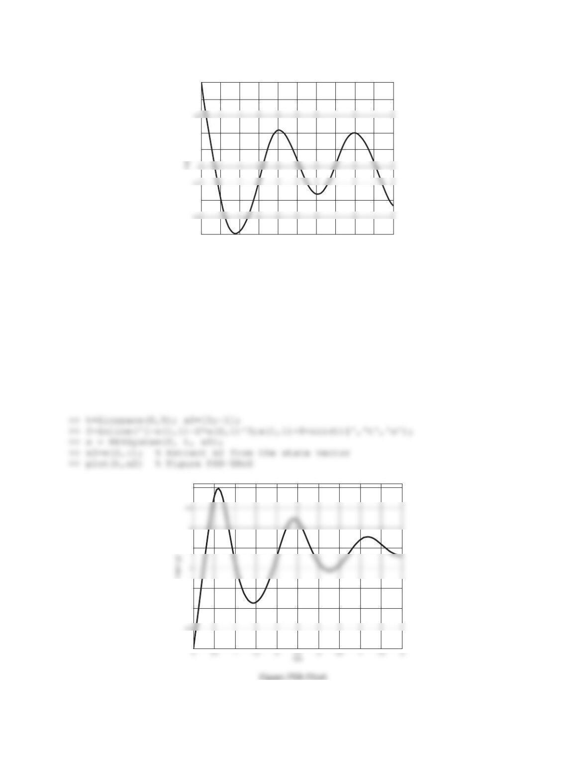
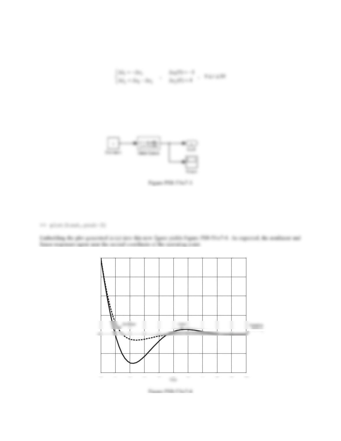
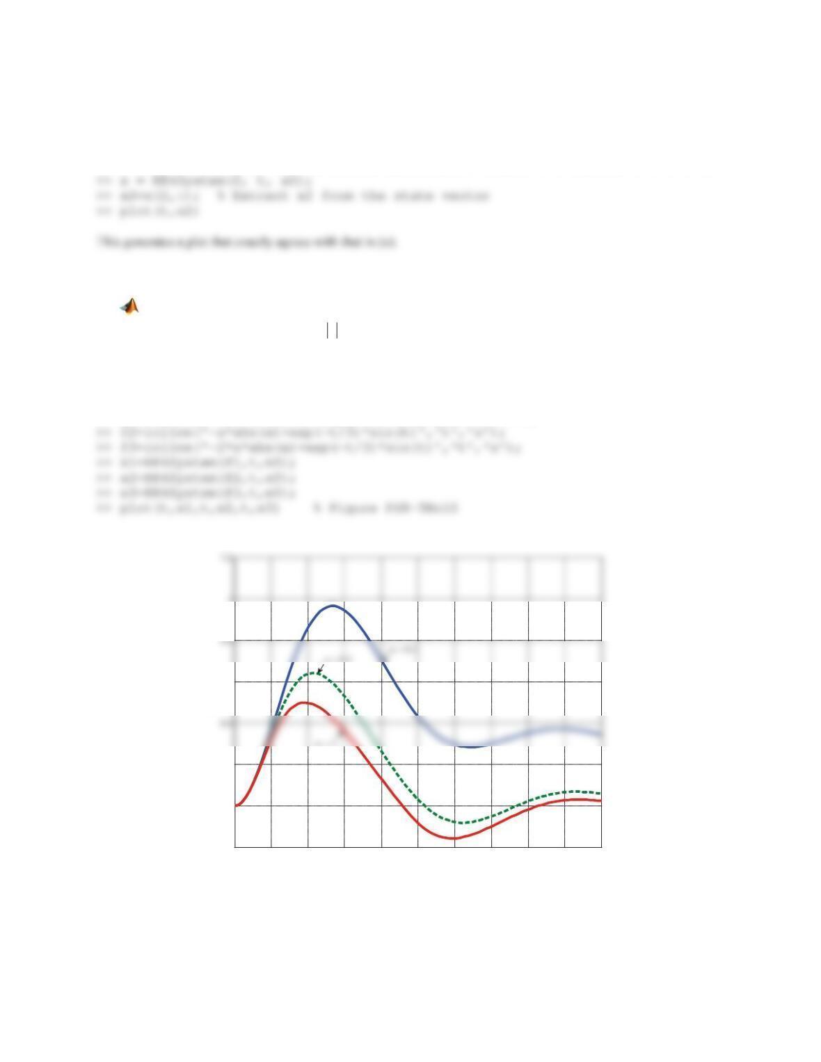
(a) Build the Simulink model and use it to generate the plot of 2()xt
.
(b) Derive the linearized model analytically. Build a Simulink model and use it to plot the time variations of the
variable in the linear model that is compatible with 2()xt
. Compare the plots generated in (a) and (b) and
comment.
Solution
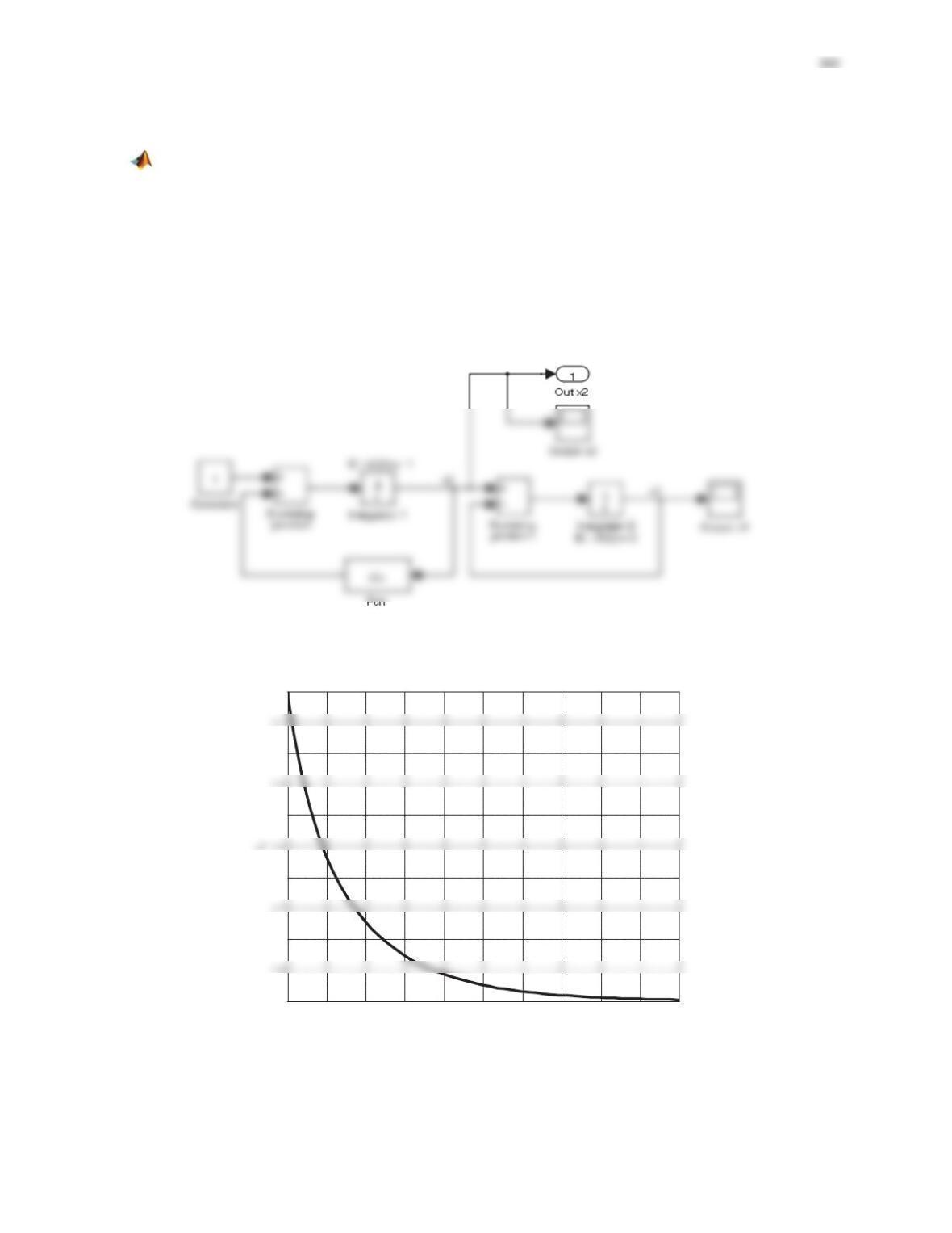
(a) The model is built and shown in Figure PS8-5No7-1. Run the simulation, followed by
>> plot(tout,yout) % Figure PS8-5No7-2
Figure PS8-5No7-1
Figure PS8-5No7-2
0 1 2 3 4 5 6 7 8 9 10
-3.5
-2.5
-1.5
-0.5
1
Time
x
359
(b) The operating point is
(0, 3)
. The linearized model is derived as
The model in Figure PS8-5No7-3 is built using the state-space matrices and initial state:
>@
0
01 0 1
, , 0 1 , 0,
11 0 4
D
ªºªº ½
®¾
«»«»
¬¼¬¼ ¯¿
ABC x
Simulate this model. The output will be 2
x'by design. But in order to get access to the second variable
compatible with 2
xin the nonlinear model, we realize that 22
3xx' . Therefore, the command that will generate
the desired plot is
-5
-4
-2
-1
0
1
x
2
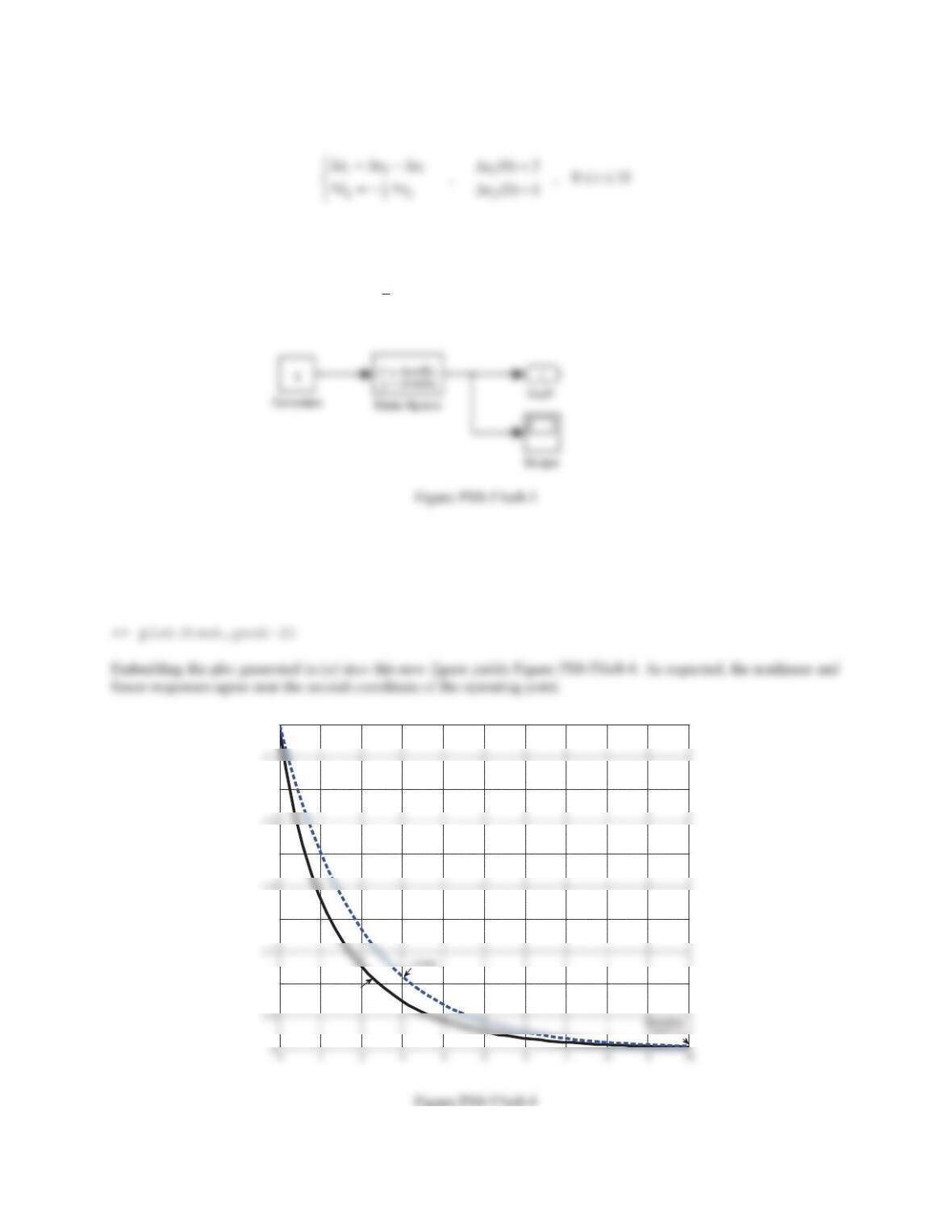
8. Repeat Problem 7 for
121 1
12
22
(0) 0
, , 0 10
(0) 1
21
xxx xt
x
xx
°dd
®
°
¯
Solution
(a) The model is built and shown in Figure PS8-5No8-1. Run the simulation, followed by
>> plot(tout,yout) % Figure PS8-5No8-2
Figure PS8-5No8-1
Figure PS8-5No8-2
0 1 2 3 4 5 6 7 8 9 10
-2
-1.8
-1.6
-1.4
-1.2
-1
Time
x
361
(b) The operating point is
(2,2)
. The linearized model is derived as
The model in Figure PS8-5No8-3 is built using the state-space matrices and initial state:
>@
0
1
2
11 02
, , 0 1 , 0,
001
D
ªº
ªº ½
®¾
«»
«»
¬¼ ¯¿
¬¼
ABC x
Simulate this model. The output will be 2
x'by design. But in order to get access to the second variable
compatible with 2
xin the nonlinear model, we realize that
22
2xx'
. Therefore, the command that will generate
the desired plot is
-1.8
-1.6
-1.4
-1.2
-1
Nonlinear
9. A nonlinear system model is derived as
12 1
3
2
21112
(0) 1
, , 0 10
(0) 1
2sin
xx xt
x
xxxxx t
°dd
®
°
¯
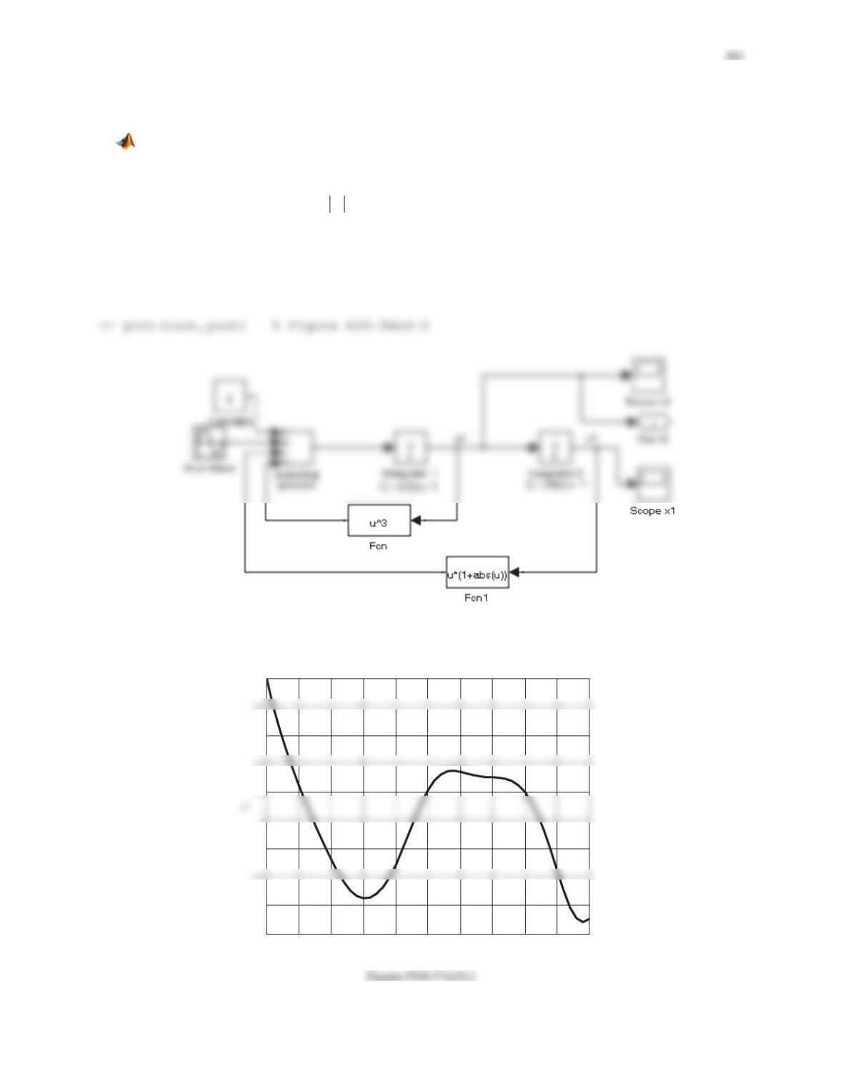
Plot 2()xt using
(a) The Simulink model of the system.
(b) The RK4 method.
Solution
(a) The model is built and shown in Figure PS8-5No9-1. Run the simulation, followed by
Figure PS8-5No9-1
0 1 2 3 4 5 6 7 8 9 10
-0.8
-0.6
-0.2
0.2
0.6
1
Time
363
(b)
>> t=linspace(0,10); x0=[-1;1];
>> f=inline('[x(2,1);-x(1,1)-x(1,1)*abs(x(1,1))-x(2,1)^3-2+sin(t)]','t','x');
10. Consider the nonlinear model
/3
2 sin , (0) 0 , 0 10
t
xaxxe t x t
dd
where
a
is a parameter. Use the RK4 method to plot
()xt
for
0.1,0.5,1a
versus
010tdd
in the same
graph.
Solution
>> x0=0; t=linspace(0,10);
>> f1=inline('-0.2*x*abs(x)+exp(-t/3)*sin(t)','t','x');
Figure PS8-5No10
0 1 2 3 4 5 6 7 8 9 10
-0.2
0
0.2
0.6
t
x(t)
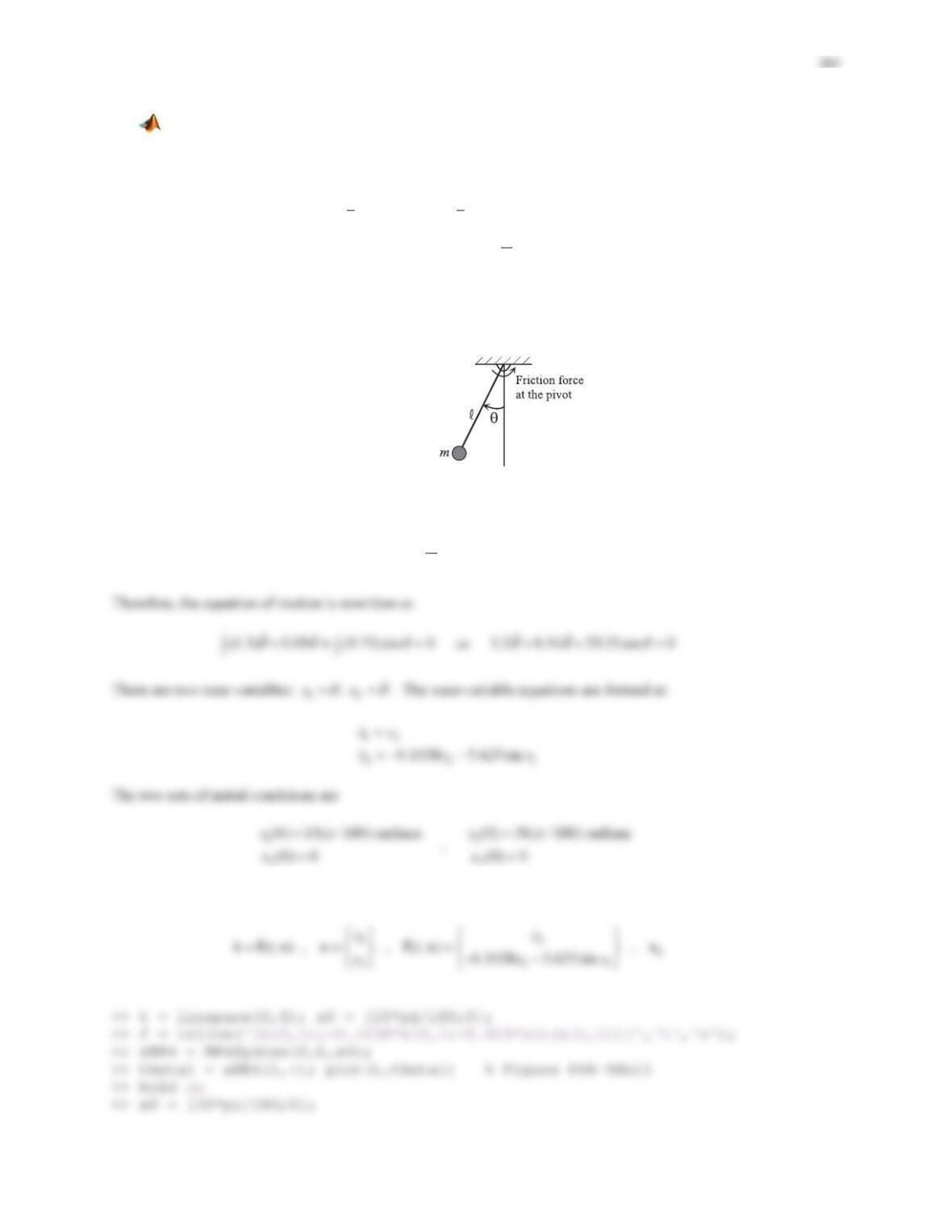
11. The pendulum system in Figure 8.35 consists of a uniform thin rod of length
l
and a concentrated mass
m
at its tip. The friction at the pivot causes the system to be damped. When the angular displacement
T
is
not very small, the system is described by the nonlinear model
2
21
32
0.09 sin 0mmg
TT T
ll
Assume, in consistent physical units, that
2
1.3, 7.5
g
m
l
l
. Two sets of initial conditions are to be
considered: (1)
(0) 15
T
D
,
(0) 0
T
, and (2)
(0) 30
T
D
,
(0) 0
T
. Using the RK4 method plot the two angular
displacements
1
T
and 2
T
corresponding to the two sets of initial conditions versus
05tdd
in the same graph.
Angle measures must be converted to radians. Use at least 100 points for plotting.
Figure 8.35 Problem 11.
Solution
We first note that
2(1.3)(7.5) 9.75
g
mg m §·
¨¸
©¹
ll
l
In vector form,


