331
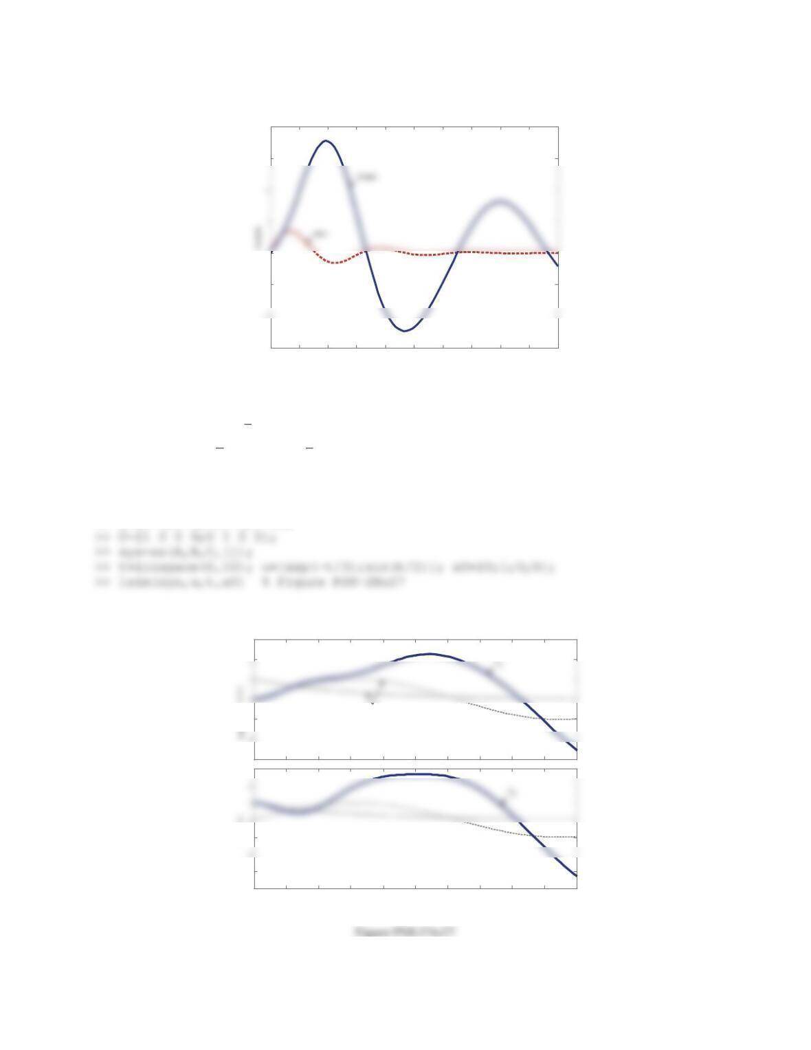
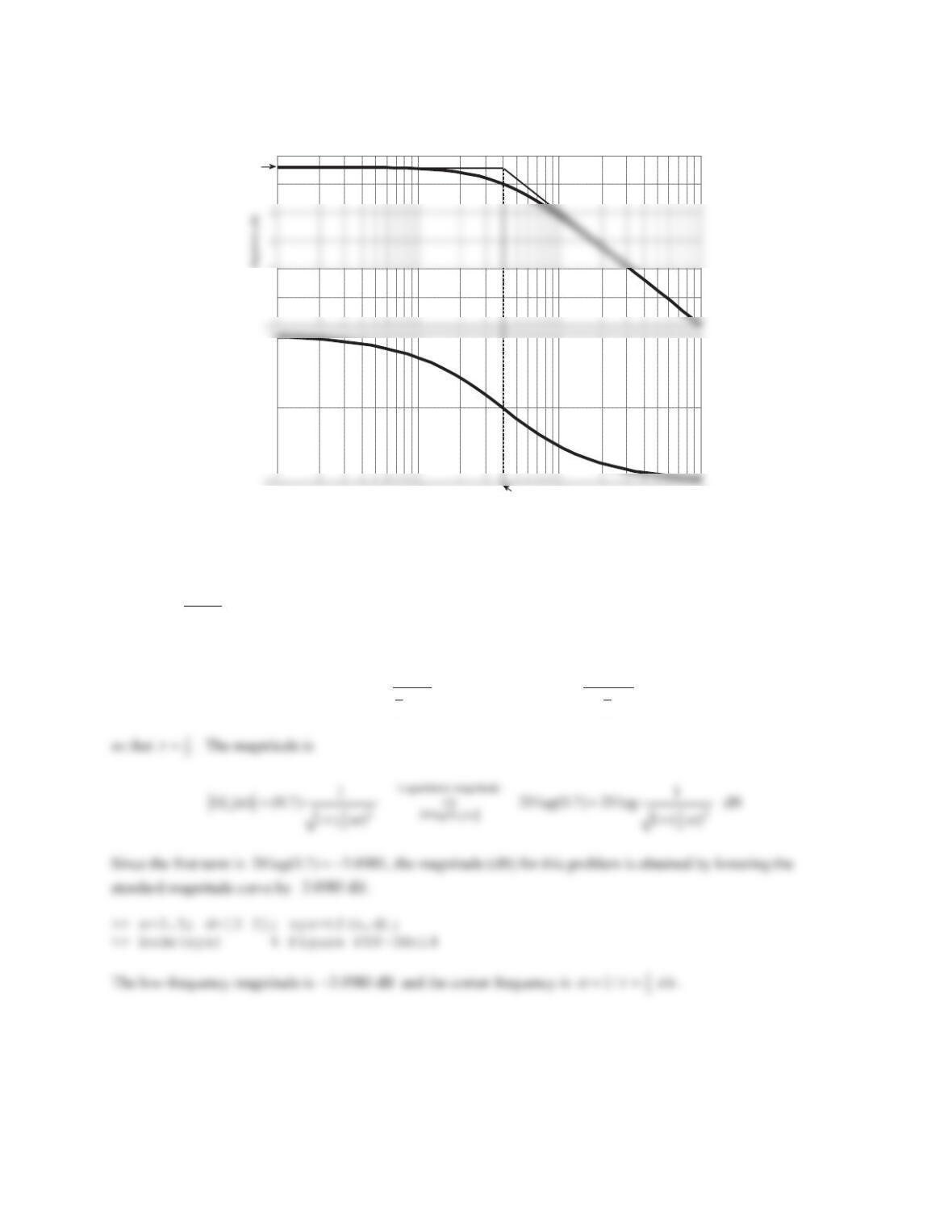
Figure PS8-2No21-1
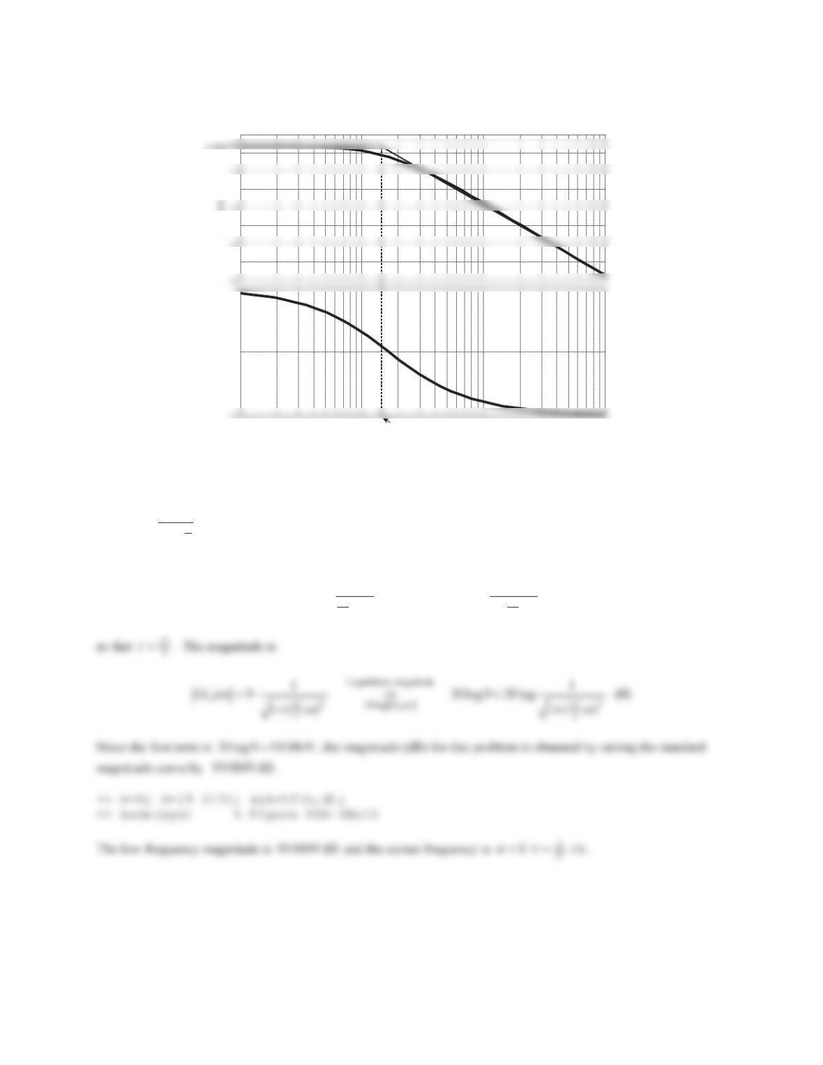
Figure PS8-2No21-2
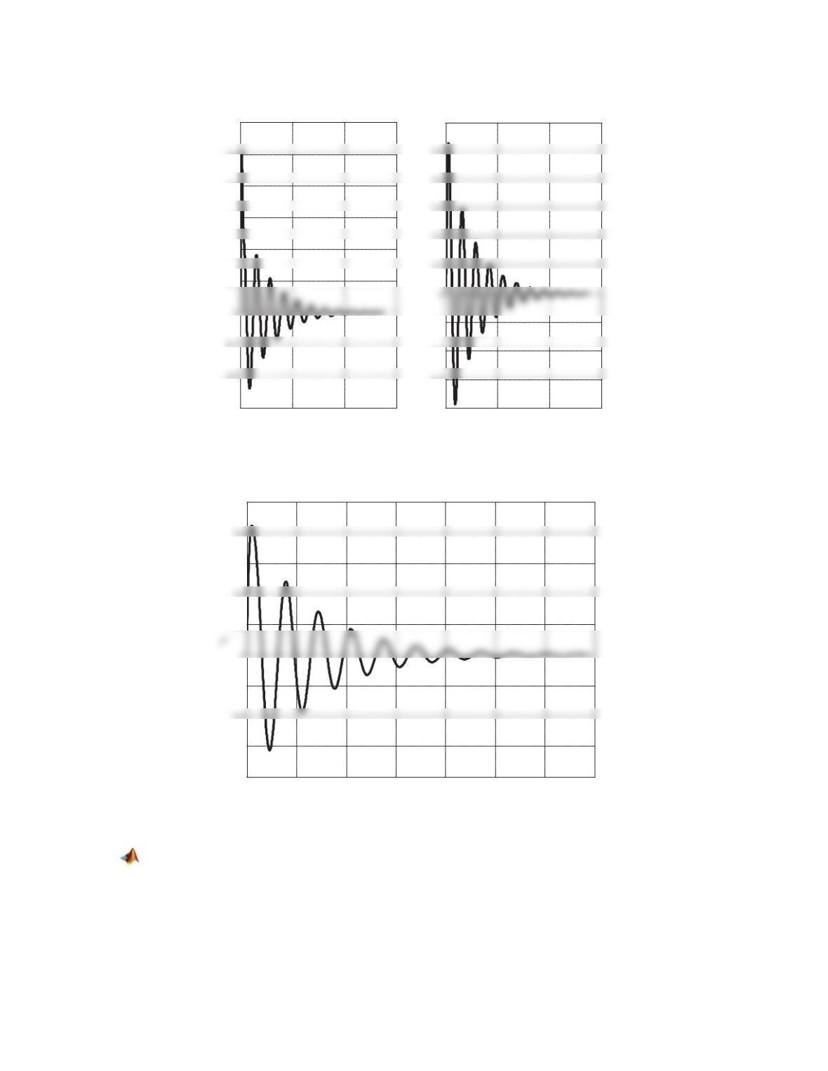
22. The equations of motion of a mechanical system are given below, where
()t
G
denotes the unit-impulse.
Assuming zero initial conditions, plot the response
1()xt
by
(a) Simulating the Simulink model of the system.
(b)Using the impulse command.
11 12
2122
22 ()
20
xx xx t
xxxx
G
°
®
°
¯
050 100 150
-0.3
0.1
0.2
0.3
0.4
0.5
0.6 Contribution of f1 to x3
050 100 150
-0.4
-0.3
-0.2
-0.1
0.6
Contribution of f2 to x3
020 40 60 80 100 120 140
-0.8
-0.6
-0.2
0.2
0.6
1
Time
332
Solution
(a) The state-space matrices are obtained as
>@
11
22
00 1 0
230, 0, 100, 0
11
D
ªºªº
«»«»
«»«»
«»«»
¬¼¬¼
ABC
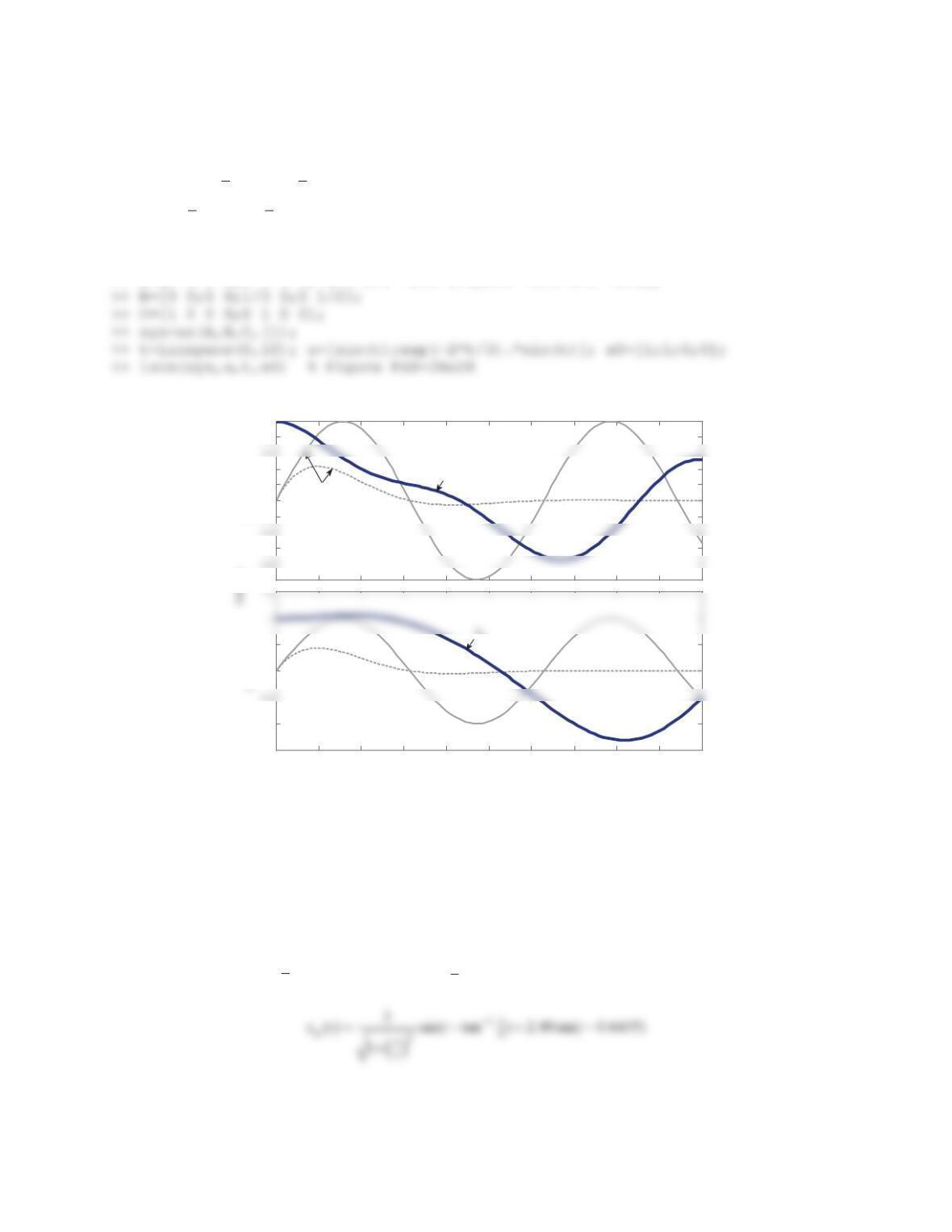
Running the simulation yields the response shown in the left tile in Figure PS8-2No22-2.
(b)
>> A=[0 0 1;2 -3 0;-1 1 -1/2]; B=[0;0;1/2]; C=[1 0 0];
Figure PS8-2No22-2
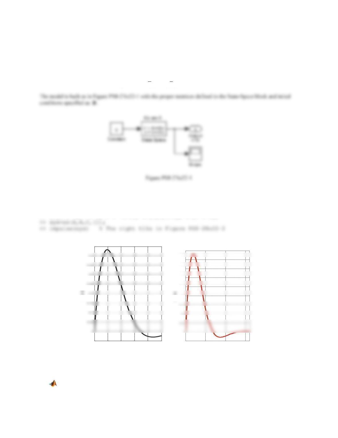
23. In Example 8.9, plot the time variations of the response 2
xby simulating the Simulink model of the system,
using the State-Space block.
0 2 4 6 8 10
-0.05
0.45
Impulse response, part (a)
Time
Amplitude
0 5 10 15
-0.05
0.2
0.25
0.3
0.35
0.4
0.45
Impulse response, part (b)
Time (seconds)
Amplitude
333
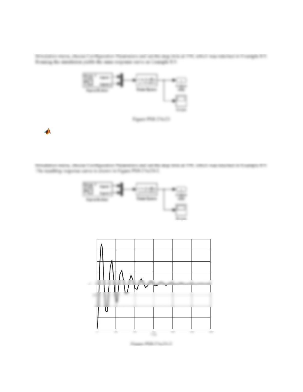
Solution
The model is built as shown in Figure PS8-2No23. The state-space matrices and the zero initial conditions are
specified in the State-Space block. The Signal Builder generates two signals, each one a unit-step. Under the
24. In Example 8.9, suppose the initial conditions are
121 2
(0) 0, (0) 1, (0) 0 (0)xxx x
. Plot the time
variations of the response 2
xby simulating the Simulink model of the system, using the State-Space block.
Solution
The model is built as shown in Figure PS8-2No24-1. The state-space matrices and the given initial conditions are
specified in the State-Space block. The Signal Builder generates two signals, each one a unit-step. Under the
Figure PS8-2No24-1
1
1.5
3.5
4
4.5
5
x
334
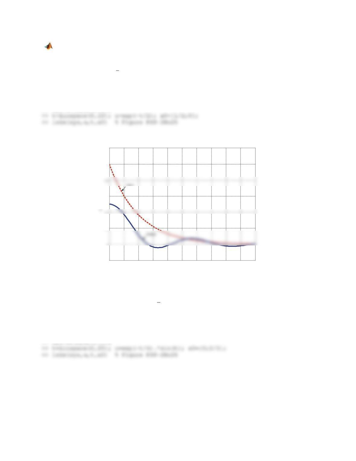
In Problems 25 through 28, the governing equations and initial conditions of a dynamic system are provided.
Plot the specified output(s) by using the lsim command.
25.
/2 1
2
2 3 , (0) , (0) 0 , 0 10
t
xx xe x x t
dd
Output : ( )xt
Solution
>> A=[0 1;-3/2 -1/2]; B=[0;1/2]; C=[1 0];
>> sys=ss(A,B,C,[]);
Figure PS8-2No25
26.
/4 2
3
8 2 10 sin , (0) 0 , (0) , 0 20
t
xx x e tx x t
dd
Output : ( )xt
Solution
>> A=[0 1;-1/4 -1/8]; B=[0;5/4]; C=[1 0];
>> sys=ss(A,B,C,[]);
0123456 78910
-0.2
0.2
0.6
1
1.2
Linear Simulation Results
Time (seconds)
335
Figure PS8-2No26
27.
/3
1
11 21 21
211
11
22
221 21
22
2 2()() (0) 0, (0) 0
, , 0 10
(0) 1, (0) 0
2( ) ( ) sin
t
xx xx xx e xx t
xx
xxx xx t
°dd
®
°
¯
12
Outputs: (), ()xt x t
Solution
>> A=[0 0 1 0;0 0 0 1;-3/2 1 -1/4 1/4;2 -2 1/2 -1/2];
>> B=[0 0;0 0;1/2 0;0 1];
0 2 4 6 8 10 12 14 16 18 20
-3
-1
0
3
4
Linear Simulation Results
Time (seconds)
-3
-1
3
To: Out(1)
0 1 2 3 4 56 78910
-4
-3
-1
3
To: Out(2)
Time (seconds)
Inputs
336
28.
21
1 1 21 21
32 11
2/3
21 22
221 21
32
32()()sin (0) 1, (0) 0
, , 0 10
(0) 1, (0) 0
2( )( ) sin
t
x x xx xx t xx t
xx
xxx xxe t
°dd
®
°
¯
12
Outputs: (), ()xt x t
Solution
>> A=[0 0 1 0;0 0 0 1;-8/9 2/9 -1/6 1/6;1/3 -1/3 1/4 -1/4];
Figure PS8-2No28
Problem Set 8.3
In Problems 1 through 8 find the frequency response of the system.
1.
3 4 12sinxx t
Solution
In standard form, we have
3
4
3sinxx t
so that 3
4
W
,
03F
, and
1 r/s
Z
. The frequency response is
-1
-0.6
-0.2
0
0.2
0.4
0.8
1
To: Out(1)
0 1 2 3 4 5 6 7 8 9 10
-1.5
-1
0
0.5
Linear Simulation Results
Time (seconds)
Inputs
x1
337
2.
1
2
210sin2xx t
Solution
In standard form, we have
420sin2xx t
so that 4
W
,
0
20F
, and
2 r/s
Z
. The frequency response is
3.4 0.9sin( / 2)yy t
Solution
In standard form, we have
1
4
0.2250sin( / 2)yy t
so that
1
4
W
,
00.2250F
, and
1
2
r/s
Z
. The frequency
response is
4.
2
3
3 19.8sin( / 3)yy t
Solution
In standard form, we have
2
9
6.6sin( / 3)yy t
so that 2
9
W
,
0
6.6F
, and
1
3
r/s
Z
. The frequency response is
given by
5.
41213 25sin2xxx t
Solution
The transfer function is
FRF
2
2
11324
( ) ( ) 3 24 585
41213
j
Gs G j j
ss
Z
Z
6.
25810sin3xxx t
Solution
The transfer function is
FRF
3
2
1 1 10 15
( ) ( ) 10 15 325
258
j
Gs G j j
ss
Z
Z
7.4 2 10 3.8sin( / 2)xx x t
Solution
The transfer function is
8.
9 0.9 20 20sin( / 3)xxx t
Solution
The transfer function is
339
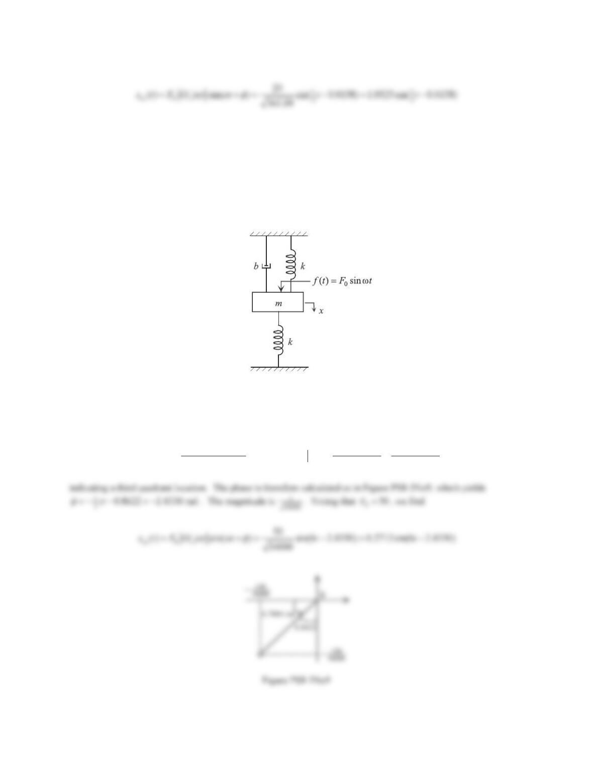
9. The equation of motion for the mechanical system in Figure 8.27isderived as
0
2sinmx bx kx F t
Z
where
x
is measured from the static equilibrium. Assuming
15 kgm
,
20 N-sec/mb
,
200 N/mk
,
0
50 NF
, and
6 rad/sec
Z
, find the system’s frequency response.
Figure 8.27 Problem 9.
Solution
The transfer function is
FRF
6
2
1 1 140 120
( ) ( ) 140 120 34000
15 20 400
j
Gs G j j
ss
Z
Z
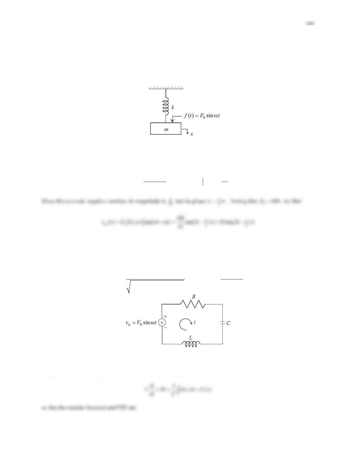
10. Find the frequency response of the mechanical system in Figure 8.28, assuming
15 kgm
,
50 N/mk
,
0
100 NF
, and
2 rad/sec
Z
.
Figure 8.28 Problem 10.
Solution
The transfer function is
FRF
2
2
11
( ) ( ) 10
15 50
Gs G j
s
Z
Z
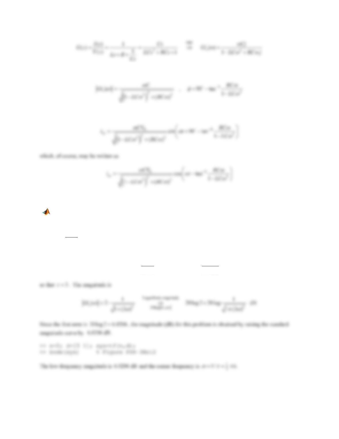
11. For the RLC circuit shown in Figure 8.29 show that the frequency response is described by
1
0
2
2
22
( ) cos tan 1
1()
ss
CV RC
it t LC
LC RC
ZZ
ZZ
ZZ
§·
¨¸
©¹
Figure 8.29 Problem 11.
Solution
Using KVL, the governing equation of the circuit is derived as
341
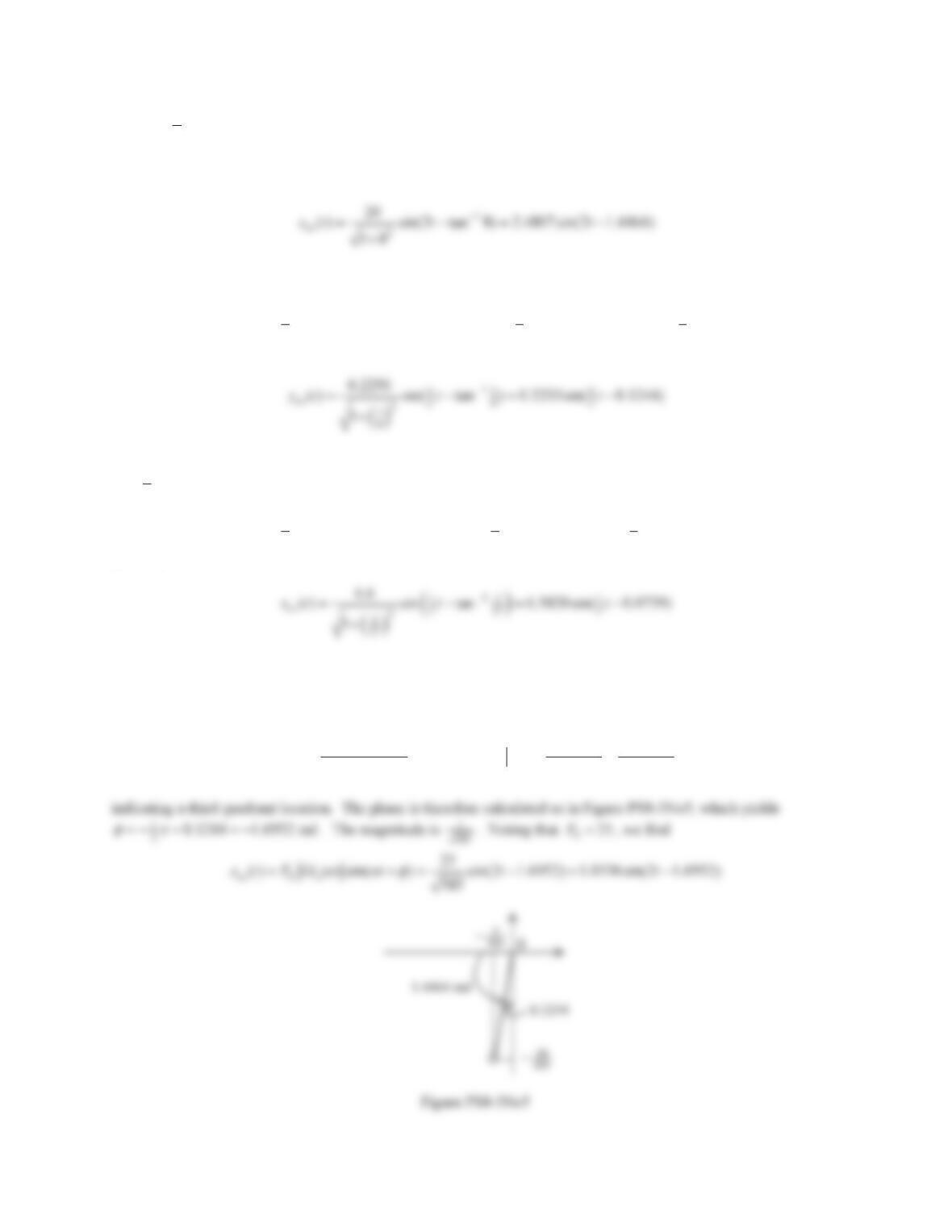
The magnitude and phase of FRF are found as
Finally, the frequency response is
In Problems 12 through 15 draw the Bode diagram and identify the corner frequency, as well as the low-
frequency magnitude (dB).
12.
2
() 31
Gs s
Solution
Rewrite as
FRF
11
( ) 2 ( ) 2
31 13
Gs G j
sj
ZZ
342
Figure PS8-3No12
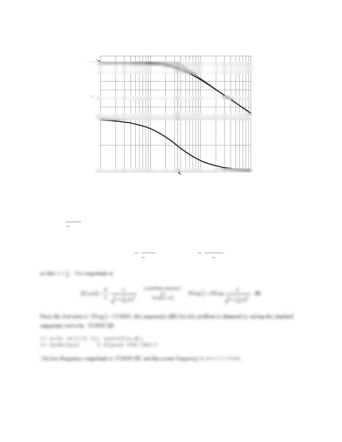
13.
1
2
9
() 2
Gs s
Solution
Rewrite as
FRF
11
44
91 9 1
( ) ( )
21 21
Gs G j
sj
ZZ
-20
-10
-5
10
10-2 10-1 100101
-45
Phase (deg)
Bode Diagram
Frequency (rad/s)
6.0206
0.33
343
Figure PS8-3No13
14.
3.5
() 35
Gs s
Solution
Rewrite as
FRF
33
55
11
( ) (0.7) ( ) (0.7)
11
Gs G j
sj
ZZ
-10
-5
10
15
10-1 100101102
-45
Phase (deg)
Bode Diagram
Frequency (rad/s)
13.0643
4
344
Figure PS8-3No14
15.
2
3
6
() 9
Gs s
Solution
Rewrite as
FRF
27 27
22
11
( ) 9 ( ) 9
11
Gs G j
sj
ZZ
-35
-25
-15
-5
0
Magnitude (dB)
10-1 100101102
-45
Phase (deg)
Bode Diagram
Frequency (rad/s)
1.67
Figure PS8-3No15
16. Show that the magnitude
2
22
1
()
1(/) (2/)
nn
Gj
Z
ZZ ]ZZ
ªº
¬¼
attains a maximum when
2
12
n
Z]
Z
.
Solution
Maximum
()Gj
Z
is achieved when
22 2
(1 ) (2 )rr
]
,/n
r
ZZ
, is minimum, which is equivalent to
minimizing
22 2
(1 ) ( 2 )rr
]
. Differentiate with respect to
r
and set equal to zero:
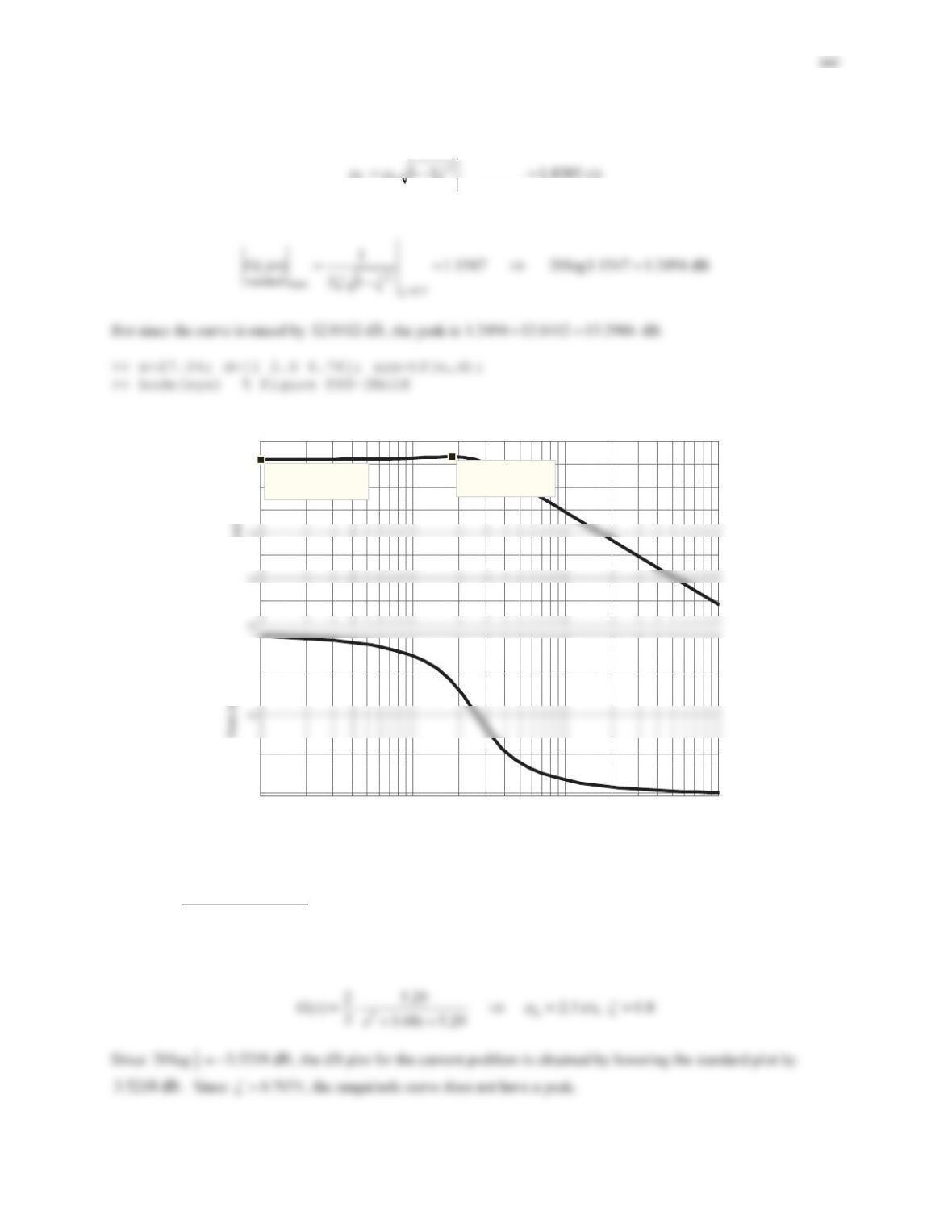
In Problems 17 through 20 draw the Bode diagram, identify the resonant frequency and find the peak
magnitude (dB), if applicable, and give the approximate low-frequency dB value.
17.
2
2
() 29
Gs ss
Solution
Rewrite
()Gs
to extract the standard, 2nd-order transfer function
-15
-5
15
10-3 10-2 10-1 100101
-90
-30
Frequency (rad/s)
0.074
19.0849
346
Since
2
9
20log 13.0643 dB
, the dB plot for the current problem is obtained by lowering the standard plot by
13.0643 dB
. Since
0.7071
]
, the magnitude curve has a peak which occurs at
n
The peak is measured as
But since the curve is lowered by
13.0643 dB
, the peak is
4.0334 13.0643 9.0309
dB.
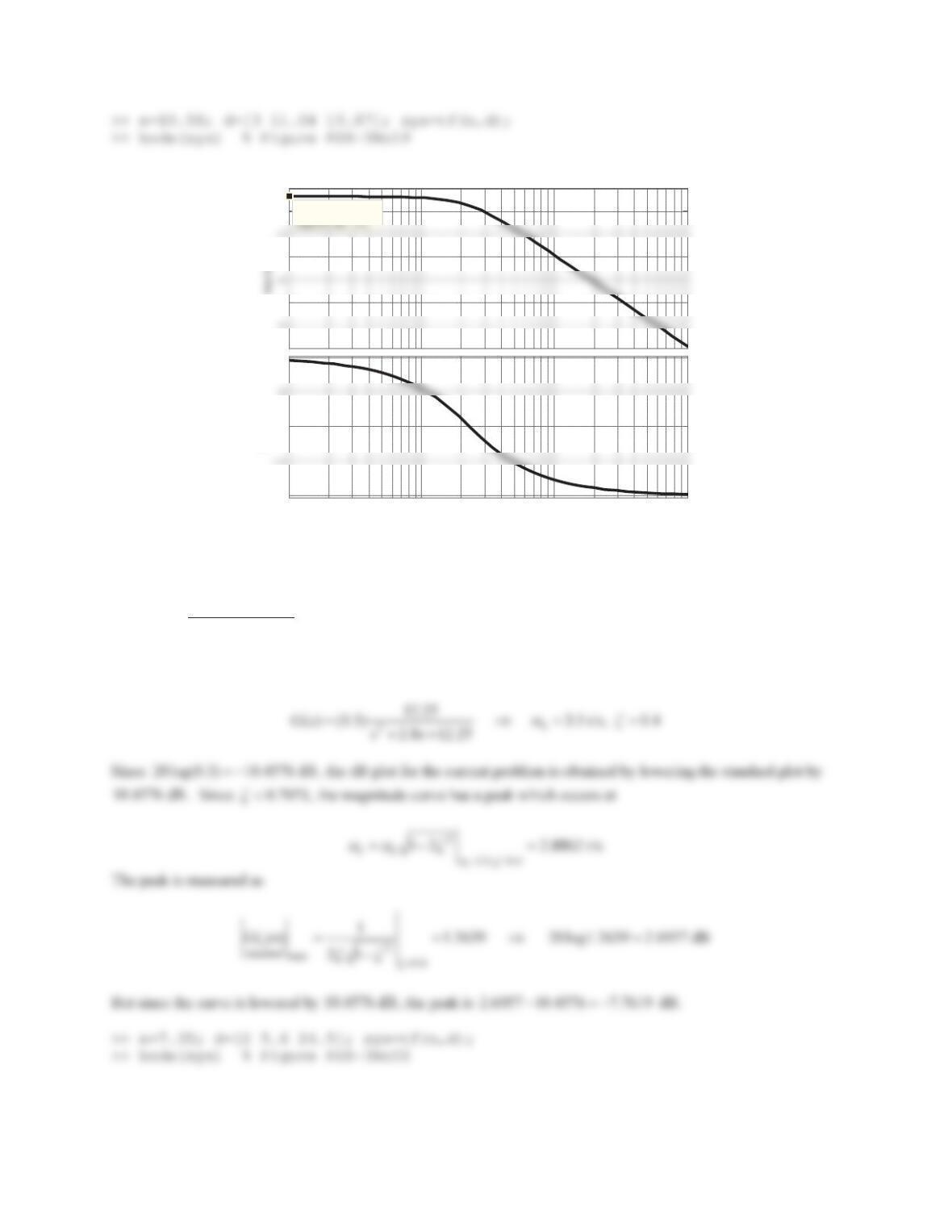
18.
2
27.04
() 2.6 6.76
Gs ss
Solution
Rewrite
()Gs
to extract the standard, 2nd-order transfer function
6.76
10-1 100101102
-180
-90
0
Phase (deg)
Bode Diagram
-80
-60
-40
-20
-10
0
System: sys
Frequency (rad/s): 2.64
Magnitude (dB): –9.03
System: sys
Frequency (rad/s): 0.101
12.0412 dB
. Since
0.7071
]
, the magnitude curve has a peak which occurs at
2.6, 0.5
n
rn
Z]
The peak is measured as
Figure PS8-3No18
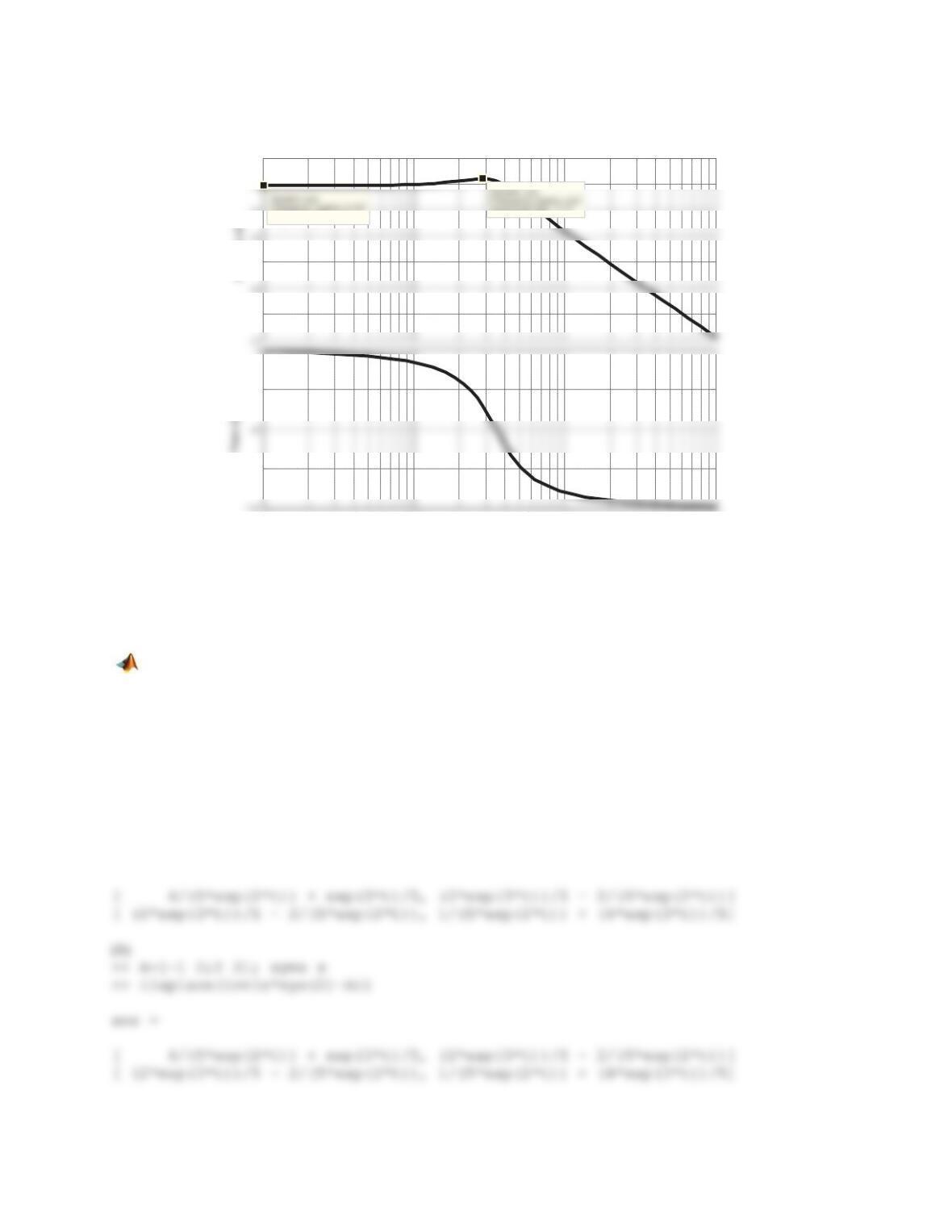
19.
2
10.58
() 3 11.04 15.87
Gs ss
Solution
Rewrite
()Gs
to extract the standard, 2nd-order transfer function
10
-1
10
0
10
1
10
2
-180
-135
-45
Bode Diagram
Frequency (rad/s)
-50
-30
-10
0
10
20
System: sys
Frequency (rad/s): 1.82
Magnitude (dB): 13.3
System: sys
Frequency (rad/s): 0.101
Magnitude (dB): 12
Magnitude (dB)
348
Figure PS8-3No19
20.
2
7.35
() 2 5.6 24.5
Gs ss
Solution
Rewrite
()Gs
to extract the standard, 2nd-order transfer function
10-1 100101102
-180
-90
0
Phase (deg)
Bode Diagram
Frequency (rad/s)
-70
-50
-30
-10
0
System: sys
Frequency (rad/s): 0.101
349
Figure PS8-3No20
Problem Set 8.4
In Problems 1 through 4, find
t
e
A
, where
A
is the matrix provided and
t
is scalar, using
(a) The expm command,
(b) The inverse Laplace-transform approach.
1.
12
22
ªº
«»
¬¼
A
Solution
(a)
>> A=[-1 2;2 2]; syms t
>> simple(expm(A*t))
ans =
10
-1
10
0
10
1
10
2
-135
-45
Bode Diagram
Frequency (rad/s)
-60
-40
-20
-10
0
Magnitude (dB): –10.5
Magnitude (dB): –7.77
Magnitude (dB)
350
2.
01
44
ªº
«»
¬¼
A
Solution
(a)
>> A=[0 1;-4 -4]; syms t
>> simple(expm(A*t))
3.
112
013
002
ªº
«»
«»
«»
¬¼
A
Solution
(a)
>> A=[-1 1 2;0 -1 3;0 0 2]; syms t
>> simple(expm(A*t))
4.
1610
2710
1610
ªº
«»
«»
«»
¬¼
A
Solution
(a)
>> A=[1 -6 10;2 -7 10;1 -6 10]; syms t