208
Figure Review5 No3
b. Taking the Laplace transform of both sides of the preceding equation with zero initial conditions results in
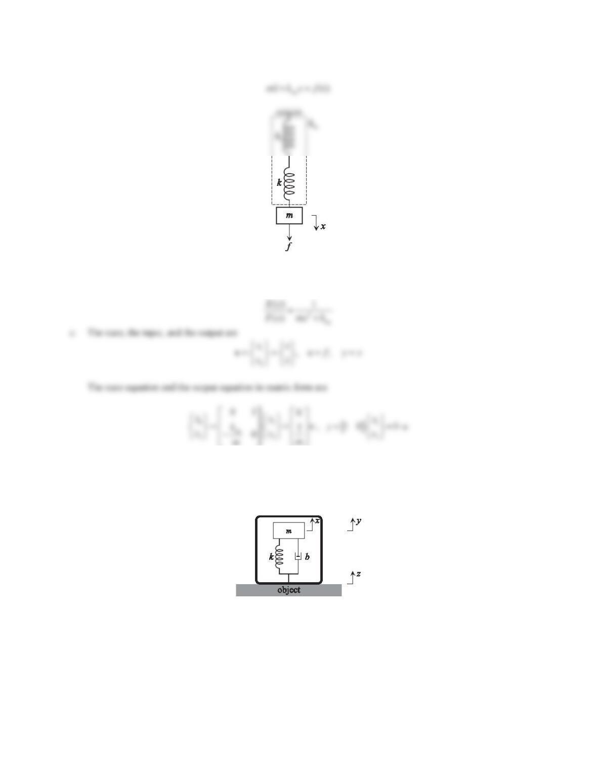
5. An accelerometer attached to an object can be modeled as a mass–damper–spring system, as shown in Figure
5.122. Denote the displacement of the mass relative to the object, the absolute displacement of the mass, and the
absolute displacement of the object as x(t), y(t), and z(t), respectively, where x(t) = y(t)–z(t) and x(t) is
measured electronically.
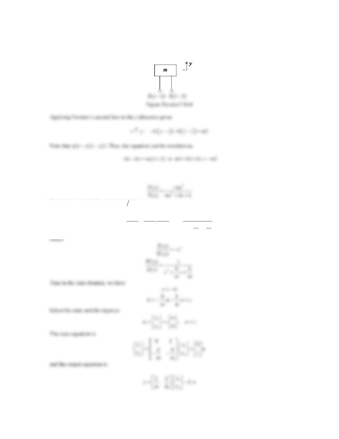
Figure 5.122 Problem 4.
a. Draw the necessary free-body diagram and derive the differential equation in terms of x(t).
b. Using the differential equation obtained in Part (a), determine the transfer function X(s)/Z(s). Assume that
the initial conditions are x(0) = 0 and
(0) 0x
.
c. Using the differential equation obtained in Part (a), determine the state-space representation. The input is
the absolute displacement of the object z(t) and the output is the displacement of the mass relative to the
object x(t).
209
Solution
a. Choose the static equilibrium as the origin of the coordinate yand assume that
0yz!!
. The free-body
diagram of the mass is shown below.
b. Assuming zero initial conditions and taking Laplace transform of the above differential equation gives
c. Rewrite the transfer function
() ()Xs Zs
as
2
2
() () () 1
() () ()
Xs XsWs sbk
Zs Ws Zs ss
mm
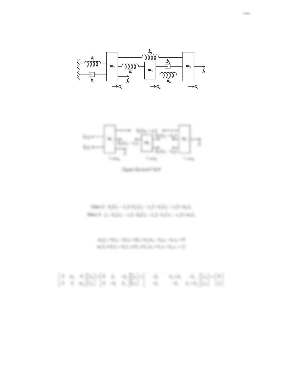
5. For the system shown in Figure 5.123, the inputs are the forces f1and f3, and the outputs are the displacements
x1,x2, and x3. Draw the necessary free-body diagrams and derive the differential equations of motion. Write the
differential equations of motion in the second-order matrix form.
Figure 5.123 Problem 5.
Solution
Choose the displacements of the three masses
1
x
,2
x, and x3as the generalized coordinates. The static equilibrium
positions of
1
m
,
2
m
, and m3are set as the coordinate origins. Assume that
321
0xxx!!!
. The free-body diagram
is shown below.
Applying Newton’s second law in the x-direction gives
:
xx
xFmao ¦
Mass 1:
1231 321 1111 11
fkxx kx x kxbxmx
Rearranging the equations, we have
11 11 1 2 3 1 32 2 3 1
()mx bx k k k x kx k x f
The differential equations can be expressed in second-order matrix form as
111 11233211
00 0 0
mxb xkkkkkxf
½ ½ ½½
ªº
ªºª º
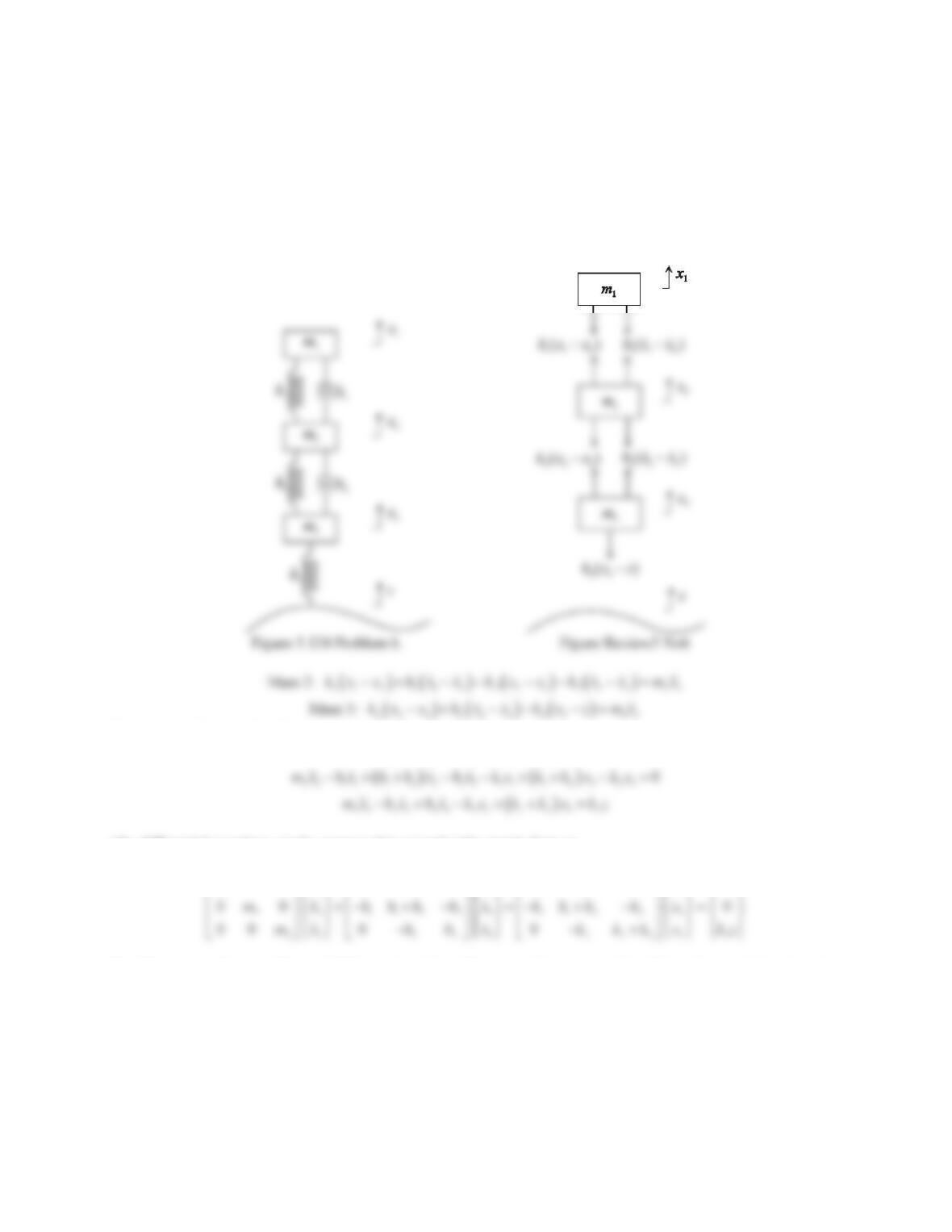
6. Consider a quarter-car model shown in Figure 5.124, where m1is the mass of the seats including passengers, m2
is the mass of one-fourth of the car body, and m3is the mass of the wheel–tire–axle assembly. The spring k1
represents the elasticity of the seat supports, k2represents the elasticity of the suspension, and k3represents the
elasticity of the tire. z(t) is the displacement input due to the surface of the road. Draw the necessary free-body
diagrams and derive the differential equations of motion. Write the differential equations of motion in the
second-order matrix form.
211
Solution
Choose the displacements of the three masses
1
x
,2
x, and 3
xas the generalized coordinates. The static equilibrium
positions of
1
m
,
2
m
, and
3
m
are set as the coordinate origins. Assume that
123
0xxxz!!!!
. The free-body
diagram is shown below. Applying Newton’s second law in the x-direction gives
:
xx
xFman ¦
Mass 1:
11 2 11 2 11
kx x bx x mx
Rearranging the equations into
11 11 12 11 12
0mx bx bx kx kx
The differential equations can be expressed in second-order matrix form as
11111111
00 0 0 0
mxbbxkk x
½ ½ ½ ½
ªº ª º
ªº
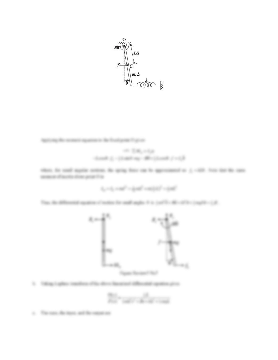
7. The system shown in Figure 5.125 consists of a uniform rod of mass mand length Land a translational spring
of stiffness kat the rod’s tip. The friction at the joint O is modeled as a damper with coefficient of torsional
viscous damping B. The input is the force fDQGWKHRXWSXWLVWKHDQJOHș7KHSRVLWLRQș FRUUHVSRQGVWRWKH
static equilibrium position when f= 0.
a. Draw the necessary free-ERG\GLDJUDPDQGGHULYHWKHGLIIHUHQWLDOHTXDWLRQRIPRWLRQIRUVPDOODQJOHVș
b. 8VLQJ WKH OLQHDUL]HG GLIIHUHQWLDO HTXDWLRQ REWDLQHG LQ 3DUW E GHWHUPLQH WKH WUDQVIHU IXQFWLRQ Ĭs)/F(s).
$VVXPHWKDWWKHLQLWLDOFRQGLWLRQVDUHș DQG
ș
.
c. Using the differential equation obtained in Part (b), determine the state-space representation.
212
Figure 5.125 Problem 7.
Solution
a. At equilibrium, we have
+ր:O0M¦
st
0k
G
st
0
G
213
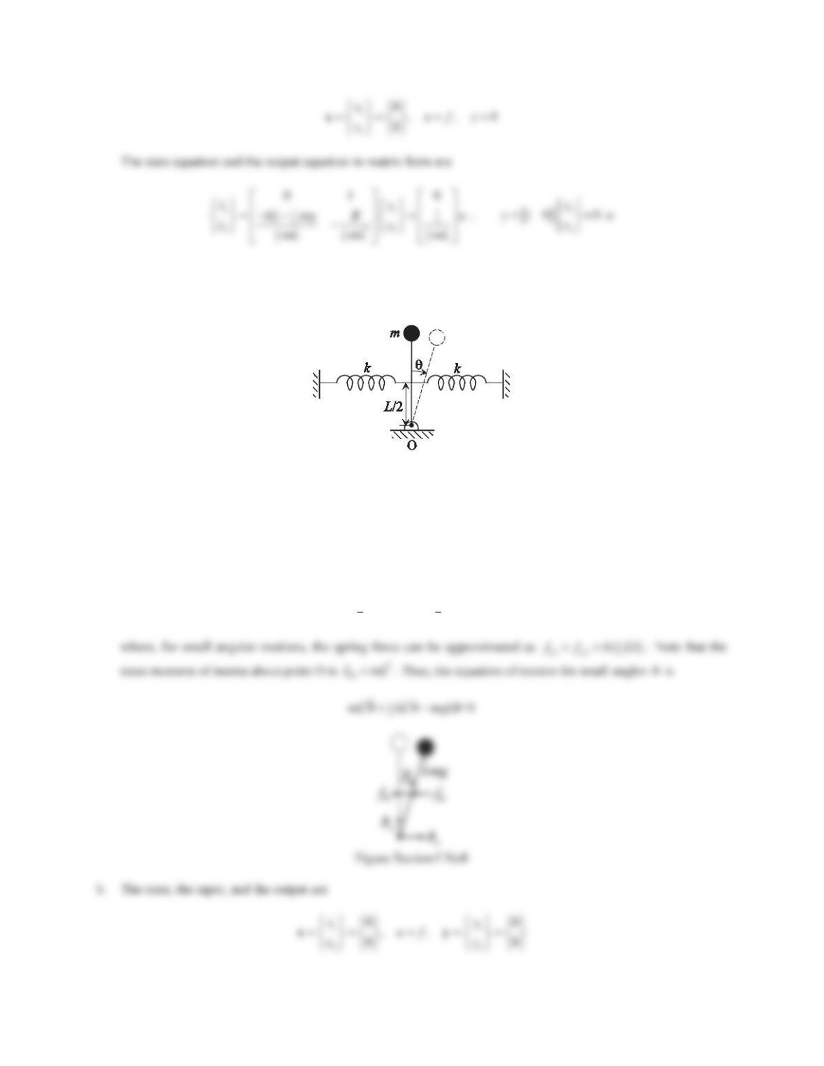
8. Consider the inverted pendulum system shown in Figure 5.126. The system consists of a bob of mass mand a
massless rod of length L. Two springs of stiffness kare connected to the middle of the rod. 7KHSRVLWLRQș
corresponds to the static equilibrium position, at which each spring is at its free length.
Figure 5.126 Problem 8.
a. Draw the necessary free-body diagram and derive the differential equatioQRIPRWLRQIRUVPDOODQJOHVș
b. Using the differential equation obtained in Part (a), determine the state-space representation. Assume that
the outputs are the angular displacement Tand the angular velocity
ș
.
Solution
a. Applying the moment equation to the fixed point O gives
+ց:
OO
ĮMI¦
11
12O
22
sin ș FRV ș FRV ș ș
kk
LmgL fL fI
214
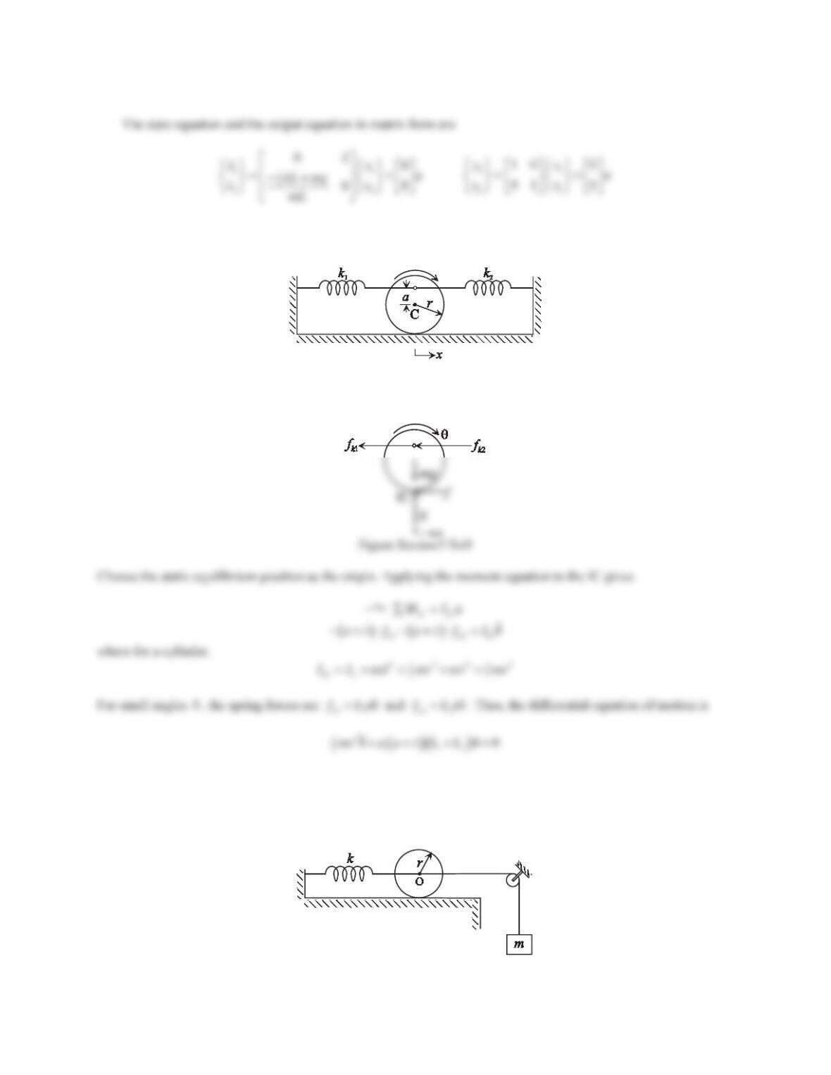
9. Consider the system shown in Figure 5.127. Assume that a cylinderof mass mrolls without slipping. Draw the
necessary free-ERG\GLDJUDPDQGGHULYHWKHGLIIHUHQWLDOHTXDWLRQRIPRWLRQIRUVPDOODQJOHVș
Figure 5.127 Problem 9.
Solution
The free-body diagram is shown in the figure below. Because the cylinder rolls without slipping, the contact point is
the IC.
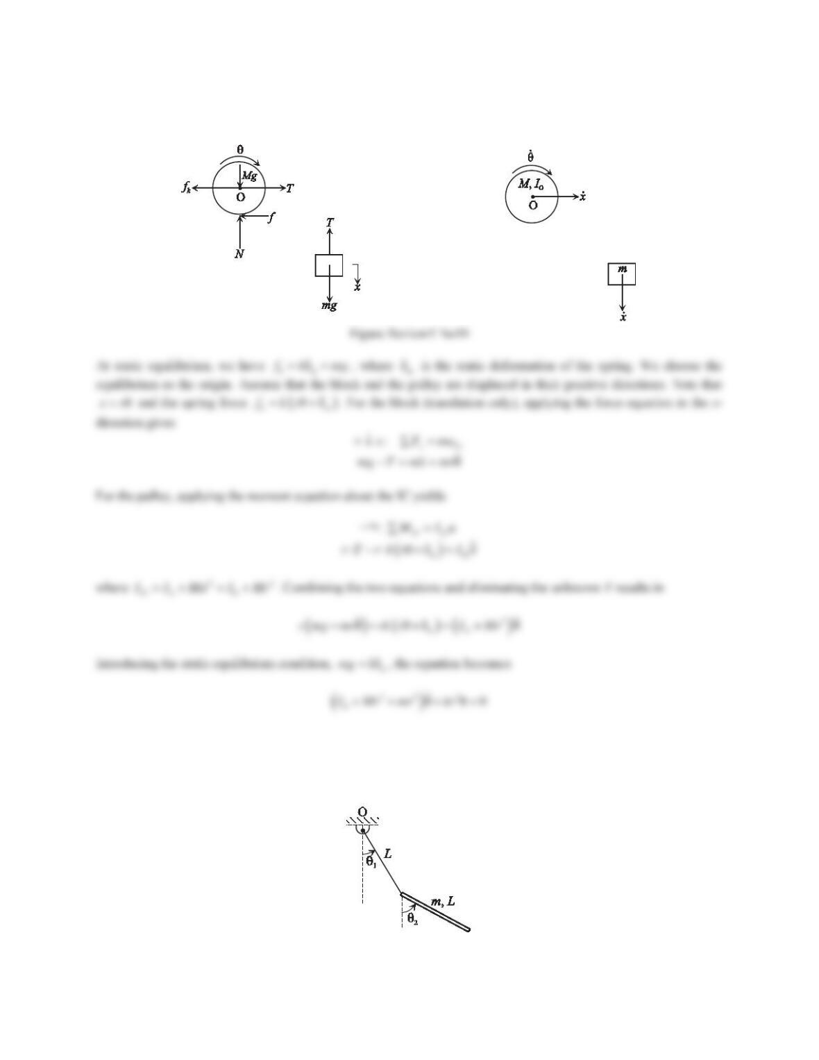
10. The pulley of mass Mshown in Figure 5.128 has a radius of r. The mass moment of inertia of the pulley about
the point O is IO. A translational spring of stiffness kand a block of mass mare connected to the pulley as
shown. Assume that the pulley rolls without slipping. Derive the equation of motion using (a) the force/moment
approach, and (b) the energy approach.
Figure 5.128 Problem 10.
215
Solution
The free-body diagram and the kinematic diagram are shown in the figure below. Because the pulley rolls without
slipping, the contact point is the IC.
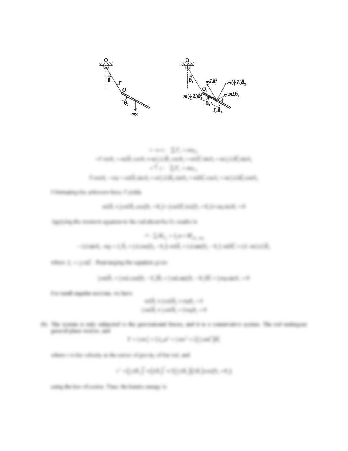
11. Consider the mechanical system shown in Figure 5.129, where a uniform rod of mass mand length Lis attached
to a massless rigid link of equal length. Assume that the system is constrained to move in a vertical plane.
‘HQRWH WKH DQJXODU GLVSODFHPHQW RI WKH OLQN DV ș1 DQG WKH DQJXODU GLVSODFHPHQW RI WKH URG DV ș2. Derive the
equations of motion for small angles using (a) the force/moment approach, and (b) the energy approach.
Figure 5.129 Problem 11.
216
Solution
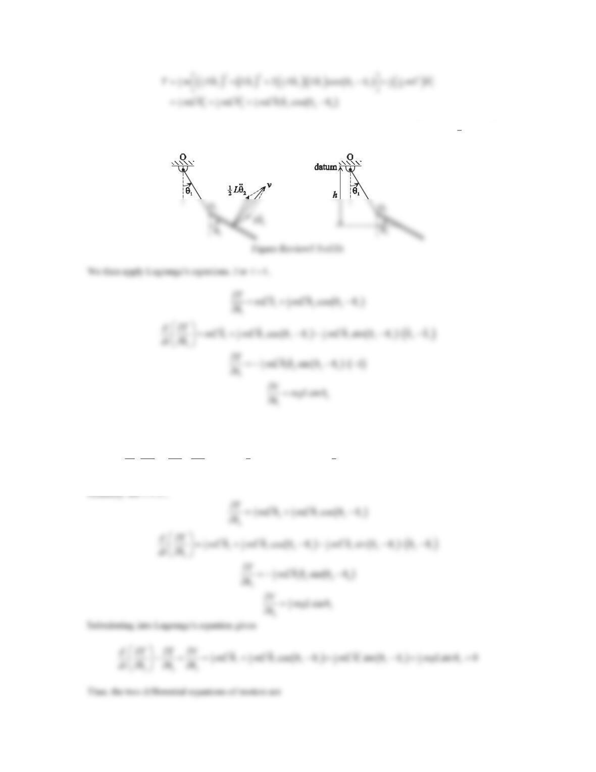
(a) The free-body diagram and the kinematic diagram are shown in the figure below.
Figure Review5 No11a
Applying the force equations to the rod gives
217
Using the datum defined in the figure, the potential energy is
1
12
2
cosșFRVș
g
VV mgh mgL L
.
Substituting into Lagrange‘s equation results in
22 22
11
1221 221 1
22
111
șșFRVșș șVLQșș VLQș
șșș
dT T V
mL mL mL mgL
dt
§·
www
¨¸
www
©¹
218
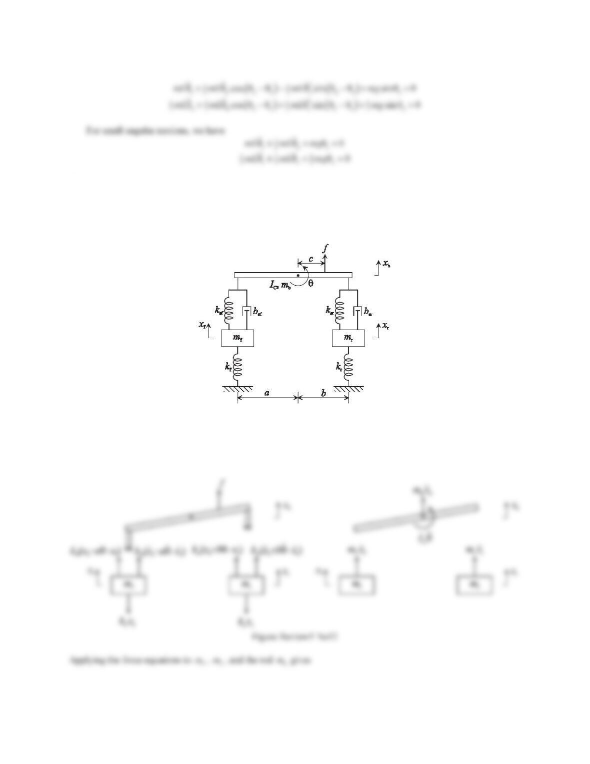
12. Consider a half-car model shown in Figure 5.130, where ICis the mass moment of inertia of the car body about
the pitch axis, mbis the mass of the car body, mfis the mass the front wheel-tire-axle assembly, and mris the
mass of the rear wheel-tire-axle assembly. Each of the front and rear wheel-tire-axle assemblies is represented
by a mass–spring–damper system. The input is the force f, and the car undergoes vertical and pitch motion.
Derive the equations of motion using the force/moment approach.
Figure 5.130 Problem 12.
Solution
Choose f
x,
r
x
,b
x,and
ș
as the generalized coordinates. The static equilibrium positions of
f
m
,
r
m
, and
b
m
are
set as the coordinate origins. Assume that
bf
șxa x!!
,
br
șxb x!!
, and
ș!
. The free-body diagram and
the kinematic diagram are shown in the figure below.
219
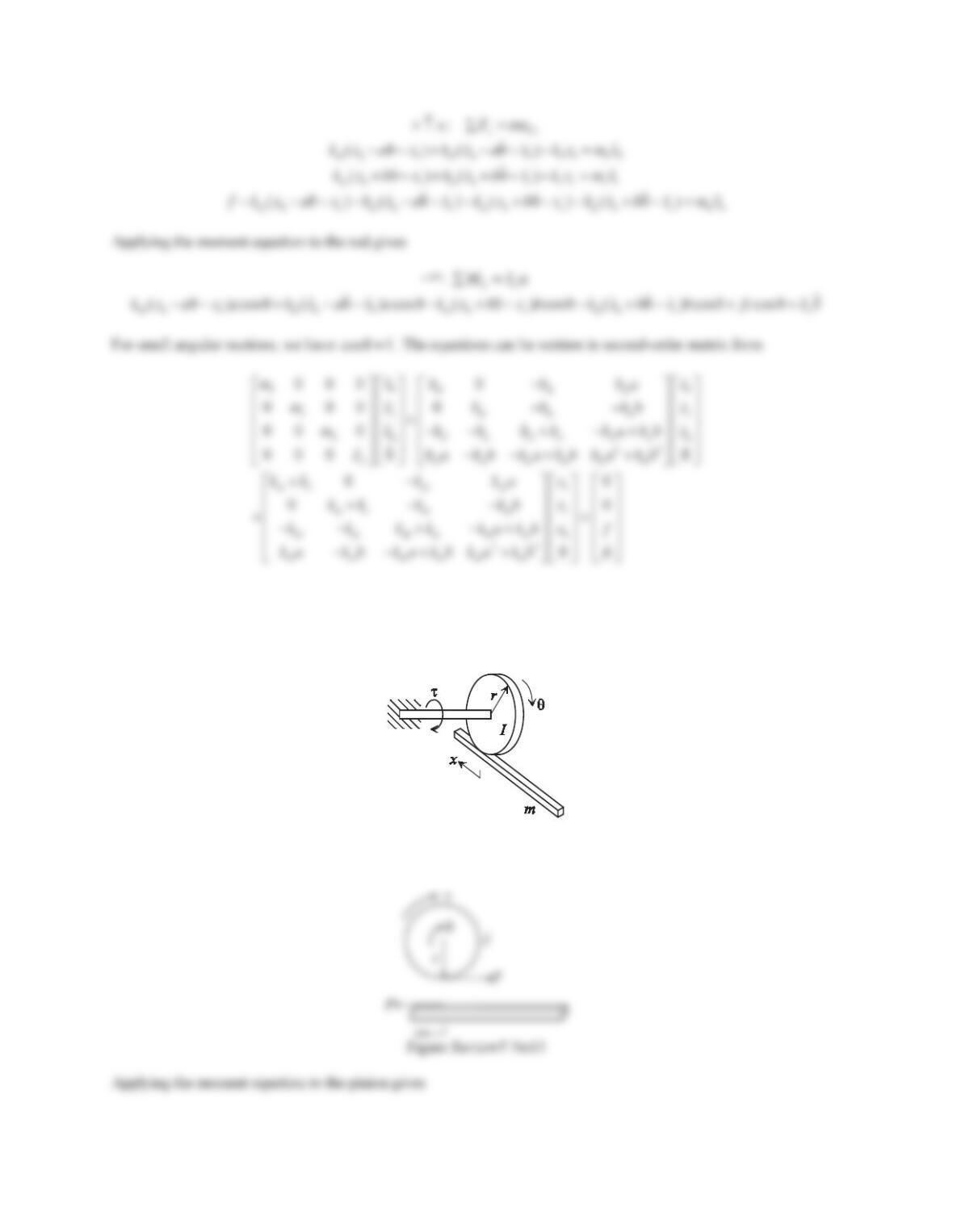
13. A rack and pinion is a pair of gears that convert rotational motion into translation. As shown in Figure 5.131, a
WRUTXHIJLVDSSOLHGWRWKHVKDIW7KHSLQLRQURWDWHVDQGFDXVHVWKHUDFNWRWUDQVODWH7KHPDVVPRPHQWRILQHUWLD
of the pinion is Iand the mass of the rack is m. Draw the free-body diagram and derive the differential equation
of motion.
Figure 5.131 Problem 13.
Solution
The free-body diagram is shown in the figure below.
220
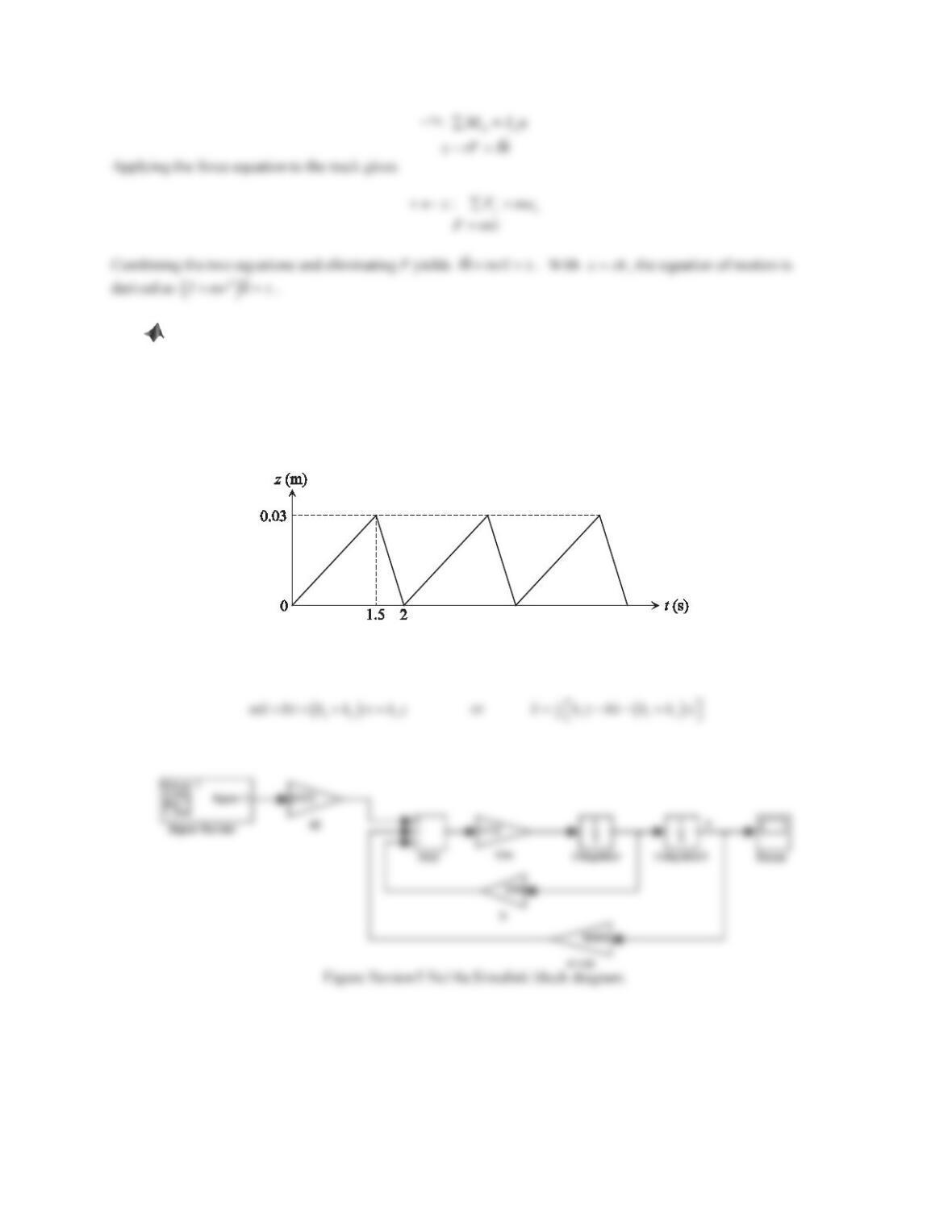
14. Consider the mass–spring–damper system shown in Problem 9 of Problem Set 5.2, where the cam and
follower impart a displacement z(t) in the form of a periodic sawtooth function (see Figure 5.132) to the lower
end of the system. The values of the system parameters are m= 12 kg, b= 200 Ns/m, k1= 4000 N/m, and k2=
2000 N/m.
a. Build a Simulink model based on the differential equation of motion of the system and find the
displacement output x(t).
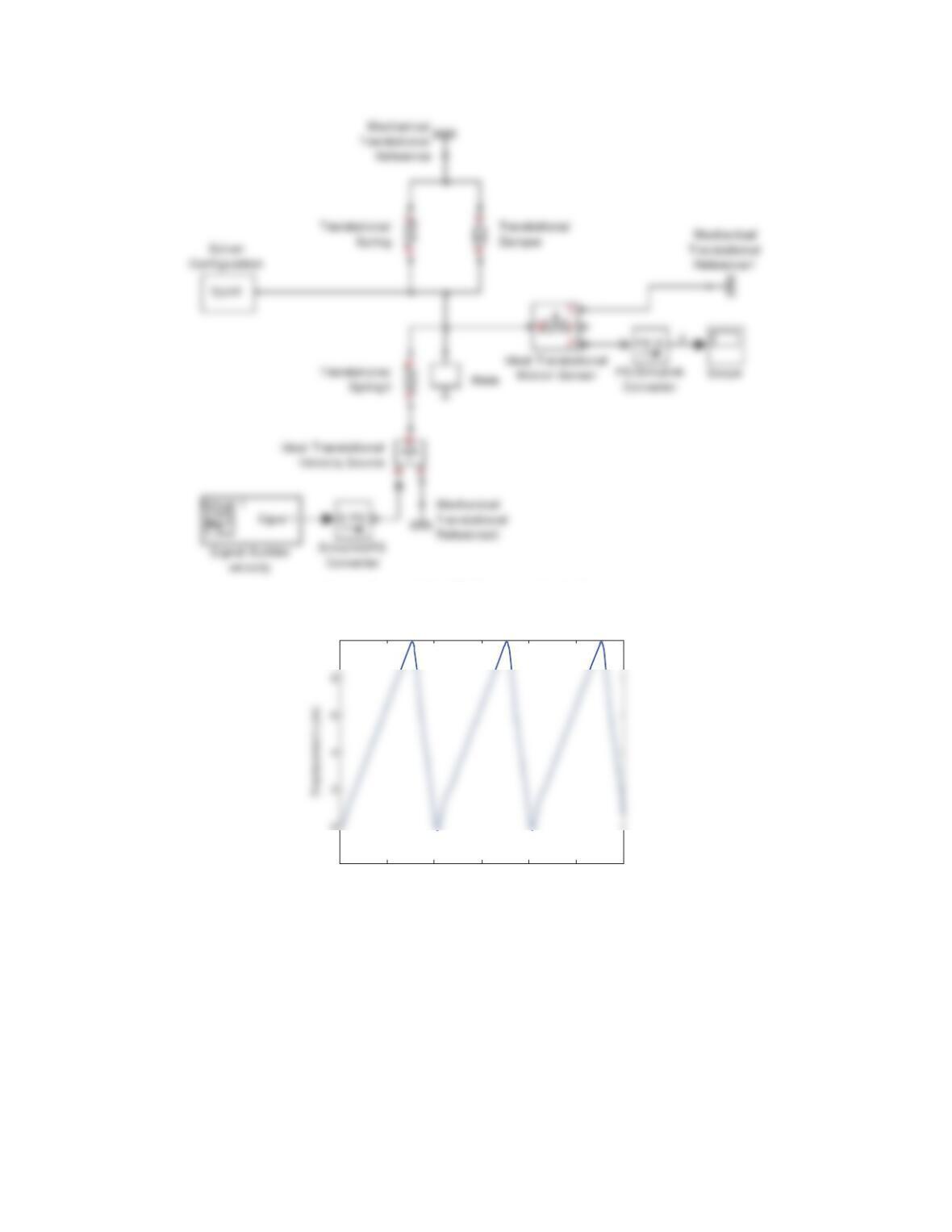
b. Build a Simscape model of the physical system and find the displacement output x(t).
Figure 5.132 Problem 14.
Solution
The differential equation of motion of the system is
221
Figure Review5 No14b Simscape block diagram.
Figure Review5 No14c
0 1 2 3 4 5 6
-2
10 x 10
-3
Time (s)