Unlock document.
This document is partially blurred.
Unlock all pages and 1 million more documents.
Get Access
65
Problem Set 4.1
In Problems 1–10 express the system model, assuming general initial conditions, in
(a) Configuration form,
(b) Standard, second-order matrix form.
1.
11 12
1
22 12
2
2( ) 10
2( ) 0
t
xx xx e
xx xx
°
®
°
¯
Solution
(a) The generalized coordinates are 11
qx and
22
qx
. Then
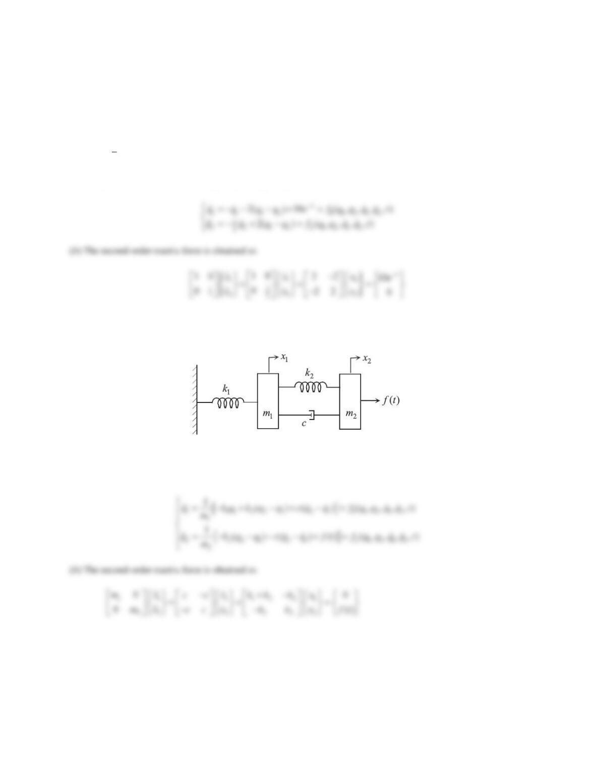
2.11 11 2 2 1 2 1
22 2 2 1 2 1
()()0
( ) ( ) ( )
mx kx k x x c x x
mx k x x cx x f t
®
¯
; Mechanical system in Figure 4.2.
Figure 4.2 Mechanical system in Problem 2.
Solution
(a) The generalized coordinates are 11
qx and
22
qx
. Then
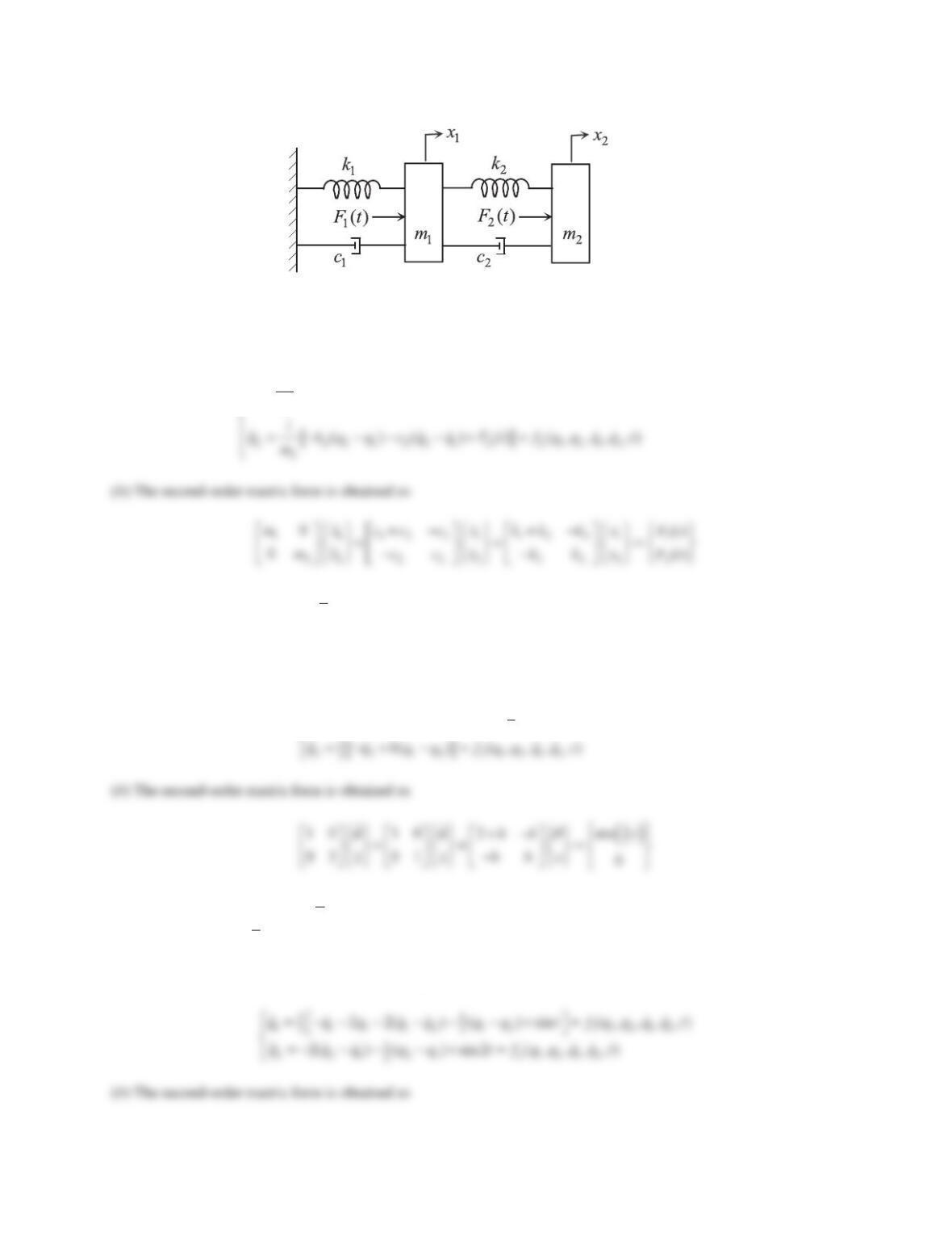
3.11 11 11 2 2 1 2 2 1 1
22 2 2 1 2 2 1 2
()()()
( ) ( ) ( )
mx cx kx k x x c x x F t
mx k x x c x x F t
®
¯
; Mechanical system in Figure 4.3.
66
Figure 4.3 Mechanical system in Problem 3.
Solution
(a) The generalized coordinates are 11
qx and
22
qx
. Then
>@
11111221221111212
1
1()()()(,,,,)
q cq kq k q q c q q Ft fqq qqt
m
°
°
4.
1
2
2()sin ( )
3 ( ) 0
bx t b const
xxb x
TT T T
T
°
®
°
¯
Solution
(a) The generalized coordinates are
1
q
T
and
2
qx
. Then
1
1 1 1 1 2 11212
2
2( )sin (,,,,)
q q q bq q t fqq qq t
°
5.
1
11 1 12 12
2
1
221 21
2
322()()sin
2( ) ( ) sin 2
II I II II t
III II t
°
®
°
¯
Solution
(a) The generalized coordinates are
11
qI
and
22
qI
. Then
67
6.
11 11 2 2 1
22 32 2 2 1
( ) 0
()()
mx kx k x x
mx kx k x x f t
®
¯
Solution
(a) The generalized coordinates are 11
qx and
22
qx
. Then
7.
1 1 21 21
232 21 21
33 32 3
( ) ( ) 0
( ) ( ) ( ) 0
( ) ( )
mx kx k x x c x x
mx k x x k x x c x x
mx kx k x x cx f t
°
®
°
¯
Solution
(a) The generalized coordinates are 11
qx ,
22
qx
, and
33
qx
. Then
>@
1 1 21 21 1123123
1( ) ( ) ( , , , , , , )
qkqkqqcqqfqqqqqqt
m
°
8.
1 1 21 21 1
232 21 21 32
3 3 32 32 2
( ) ( ) ( )
( ) ( ) ( ) ( ) 0
( ) ( ) ( )
mx kx k x x c x x F t
mx k x x k x x c x x c x x
mx kx k x x c x x F t
°
®
°
¯
Solution
(a) The generalized coordinates are 11
qx ,
22
qx
, and
33
qx
. Then
68
9.
11 12
1212
3
3( ) sin
3( ) 0
t
xx xx e t
xxx
°
®
°
¯
Solution
(a) Using the second equation, express
9
21
10
xx
and insert into the first equation to find
3
11 1
10 sin
t
xx xe t
10.
1
2
( ) xftx
x
MMM
°
®
°
¯
Solution
(a) The generalized coordinates are
1
qx
and 2
q
M
. Using the expression for x
given by the first equation in
the second equation, the configuration form is found as
Problem Set 4.2
In Problems 1–8 find a suitable set of state variables, derive the state-variable equations, and form the state equation.
1.
/3 , 0
t
x kx e k const
!
Solution
The ODE is second-order in
x
, therefore two initial conditions, (0)xand (0)x
, are needed. Thus, there are two
2.
23sinxx x t
Solution
The ODE is second-order in
x
, therefore two initial conditions, (0)xand (0)x
, are needed, and there are two state
variables:
1
xx
,
2
xx
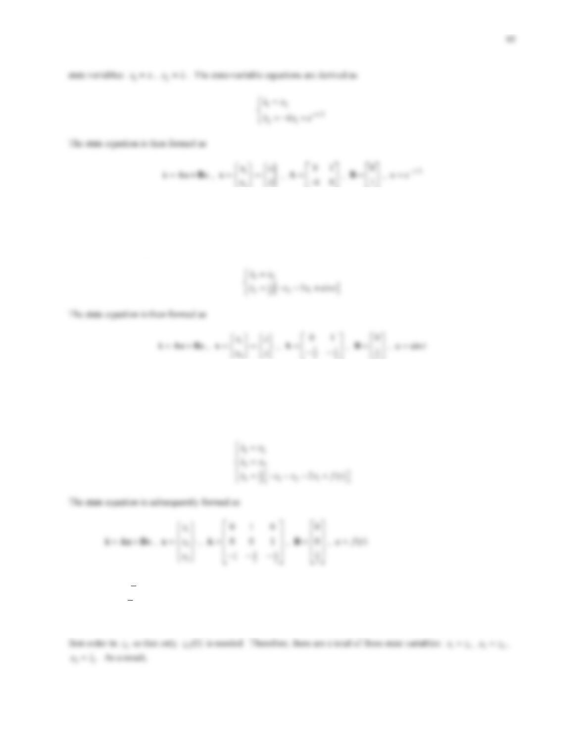
. The state-variable equations are derived as
3.
22()xxx x ft
Solution
The ODE is third-order in
x
, therefore three initial conditions, (0)x,(0)x
,(0)x
, are needed, and there are three
state variables:
1
xx
,
2
xx
,
3
xx
. The state-variable equations are then derived as
4.
1
11 121
2
1
22 21 2
2
2( )()
()()
zz zz ft
zz zz ft
°
®
°
¯
Solution
The first ODE is second-order in
1
z
, hence two initial conditions, 1(0)z,1(0)z
, are needed. The second one is
70
5.
2
3 ( )
xxx z
zzxft
®
¯
Solution
The first ODE is second-order in
x
, hence two initial conditions, (0)x,(0)x
, are needed. The second one is first-
order in zso that only (0)zis needed. Therefore, there are a total of three state variables:
1
xx
,
2
xz
,
3
xx
.
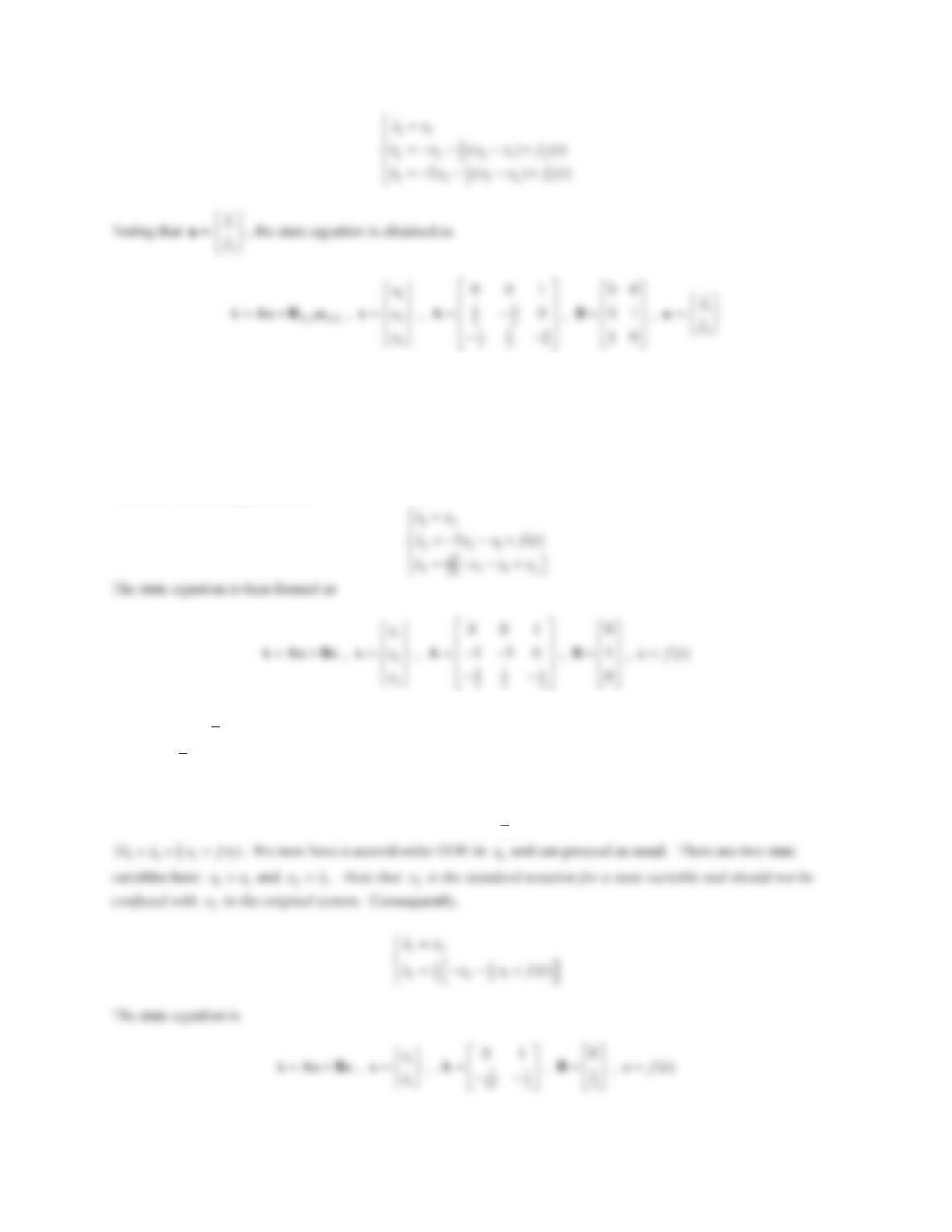
The state-variable equations are
6.
2
11 12
3
2
212
3
3()()
( ) 0
xx xx ft
xxx
°
®
°
¯
Solution
Because the second equation is algebraic, variables
1
x
and 2
xare linearly dependent, hence cannot be selected as
state variables. Solve the second equation for 2
xto find
2
21
5
xx
and insert into the first equation to obtain
71
7.
11 12
212
()
,
( )
t
zzkzz e k const
zkzz
°
®
°
¯
Solution
Because the second equation is algebraic, variables
1
z
and 2
zare linearly dependent, hence cannot be selected as
state variables. Solve the second equation for 2
zto find
21
1
k
k
zz
and insert into the first equation to obtain
8.11 12 2 1
21 12 2 2
23()
223()
xx xx x ft
xx xx x ft
®
¯
Solution
The two second-order ODEs require a total of four initial conditions for complete solution, hence there are four state
variables. We choose them as 11
xx ,
22
xx
,31
xx , and
42
xx
. Then,
9. A nonlinear dynamic system is mathematically modeled as
3/2
1
3
2sin
t
xxxe t
. Derive the state-variable
equations and express them in vector form.
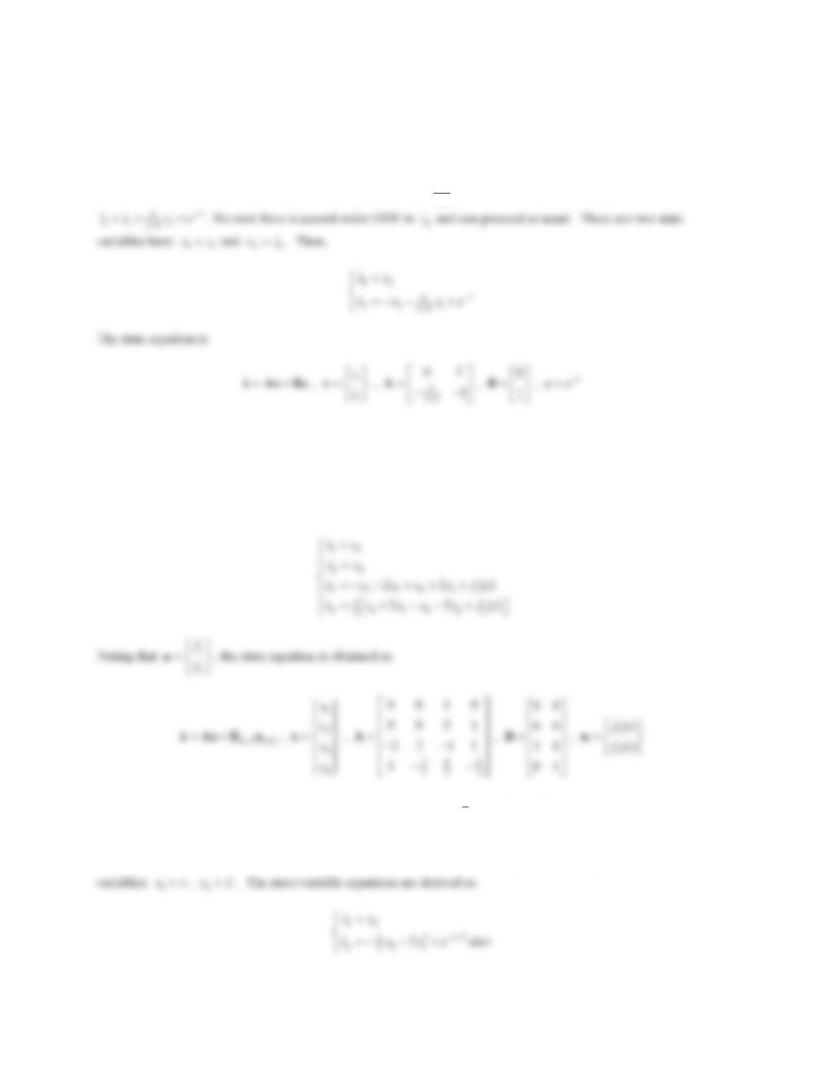
Solution
The ODE is second-order in
x
, therefore two initial conditions, (0)xand (0)x
, are needed, and there are two state
10. The mathematical model of a nonlinear system is given below. Derive the state-variable equations and express
them in vector form.
3
11 2
1
21
2
2
sin
xx x
xx t
°
®
°
¯
Solution
The first ODE is second-order in
1
x
, hence two initial conditions, 1(0)x,1(0)x
, are needed. The second one is
first-order in
x
so that only
is needed. Therefore, there are a total of three state variables: 11
xx ,
xx
,
Problems 11–14 are concerned with the stability of systems. A linear dynamic system is called stable if the
homogeneous solution of its mathematical model, subjected to the prescribed initial conditions, decays. More
practically, a linear system is stable if the eigenvalues of its state matrix all have negative real parts, that is, they all
lie in the left half-plane.
11. Determine the range of values of
k
for which the system in Problem 1 is stable.
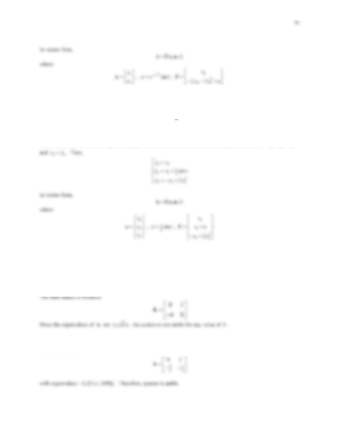
Solution
12. Decide whether the system in Problem 2 is stable.
Solution
The state matrix is
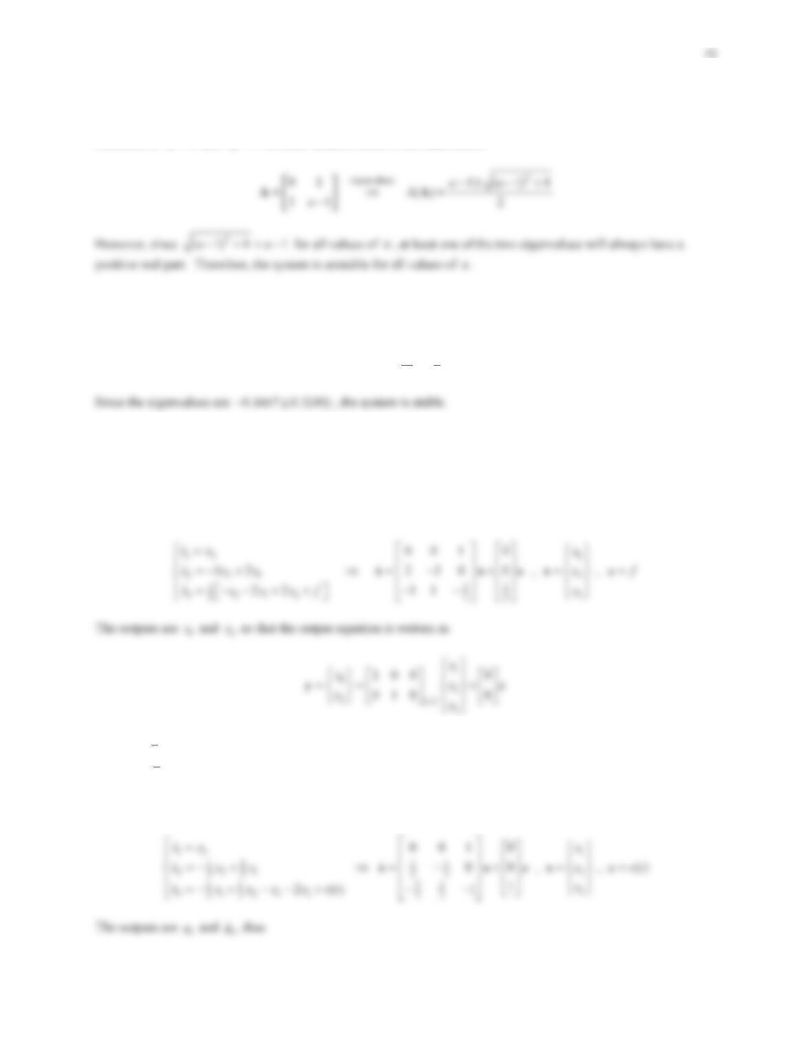
13. Find the range of values of
a
for which a system described by (1)za zzf
is stable.
Solution
Selection of 1
xz and
xz
as state variables leads to the state matrix
14. Determine whether the system in Problem 6 is stable.
Solution
The state matrix is
21
15 3
01
ªº
«»
¬¼
A
In Problems 15–18 find the state-space form of the mathematical model
15.
11 12
22 12
22()()
2( ) 0
xx xx ft
xx xx
®
¯
, outputs are
1
x
and 2
x.
Solution
Choosing state variables 11
xx ,
22
xx
,31
xx , the state-variable equations are obtained as
16.
1
11211
3
1
221
3
()2()
( ) 0
qqqqqvt
qqq
°
®
°
¯
, outputs are
1
q
and
1
q
.
Solution
With state variables 11
xq ,
22
xq
,
31
xq
, we find
74
17.
1
113 21 21
2
1
221 21
2
313
2()2()()()
2( ) ( ) 0
2( ) 0
xxx xx xxft
xxx xx
xxx
°
®
°
¯
,outputs are 2
xand 2
x
.
Solution
The third equation is algebraic. Solving for 3
xyields
2
31
3
xx
. Using this, eliminate 3
xin the first equation, while
the second equation remains as is. Then
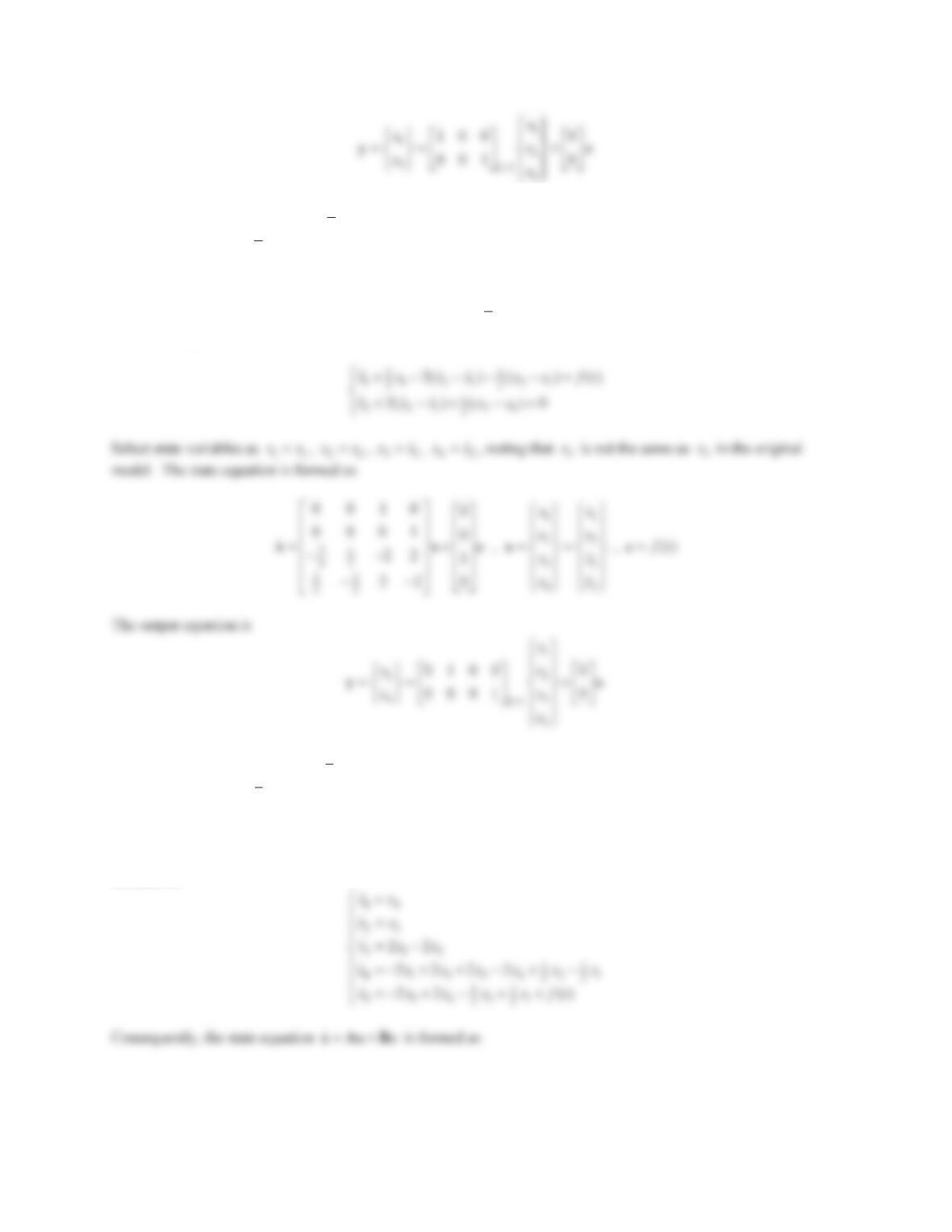
18.
1
113 21 21
2
1
221 21
2
313
2()2()()0
2( ) ( ) ( )
2( )
xxx xx xx
xxx xxft
xxx
°
®
°
¯
, outputs are
1
x
and 3
x.
Solution
There are five state variables: 11
xx ,
22
xx
,
33
xx
,
41
xx
,
52
xx
. The state-variable equations are then
obtained as
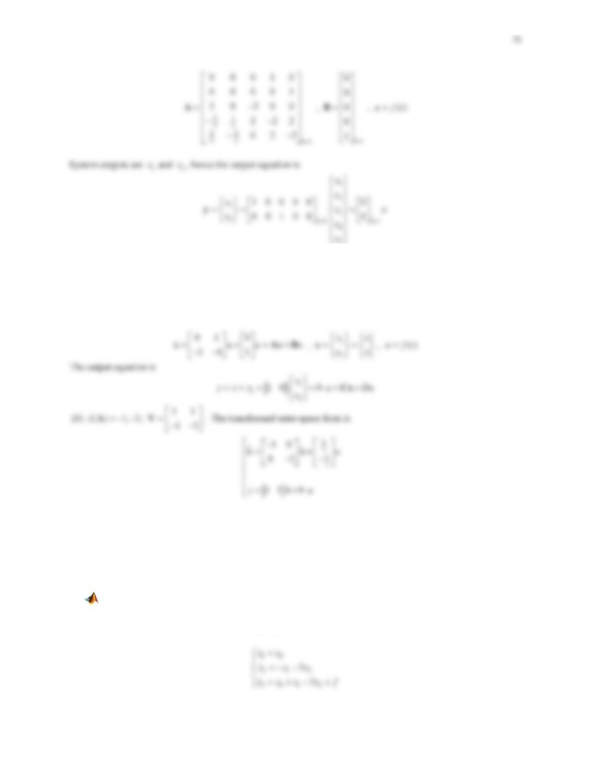
19. A dynamic system model is described by 43 ()xxxft
, where
x
is the output.
(a) Find the state-space form.
(b) Decouple the state equation and obtain the transformed state-space form.
Solution
(a) The state equation is
20. The governing equations for a system are given as
111 2
212
3()
3
xxx x ft
xxx
®
¯
where the outputs are
1
x
and
1
x
.
(a) Find the state-space form.
(b) Decouple the state equation obtained in (a) and present the transformed state-space form.
Solution
(a) There are three state variables 11
xx ,
22
xx
,31
xx , which lead to
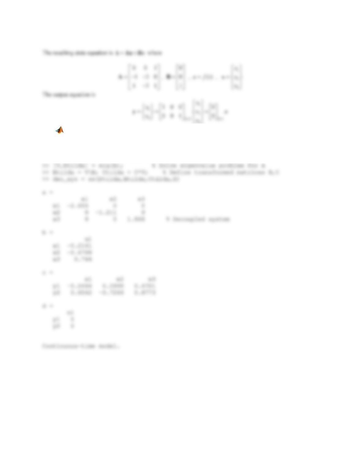
76
3
¯¿
(b)
% Define state-space form matrices A,B,C,D
>> A = [0 0 1;-1 -3 0;1 -3 1];
>> B = [0;0;1]; C = [1 0 0;0 0 1]; D = [0;0];
Problem Set 4.3
In Problems 1–8 find all possible input-output equations.
1.
1112
2212
()
20
xxxx ft
xxxx
®
¯
,()ft=input, 2
x=output
Solution
One input-output equation is expected. Laplace transformation of the original system leads to
77
2
12
2
12
(1)()()()
() ( 2 1) () 0
ss XsXsFs
Xs s s X s
°
®
°
¯
2.
11 12
22 12
2( ) 0
2( ) ( )
xx xx
xx xx ft
®
¯
,()ft=input,
1
x
=output
Solution
One input-output equation is expected. Laplace transformation of the original system leads to
2
12
2
12
( 2) ( ) 2 ( ) 0
2 () ( 2) () ()
ss Xs Xs
Xs s s X s Fs
°
®
°
¯
3.
11 1 2 1
2122
2( ) ( )
2( ) ( )
xx xx ft
xxxft
®
¯
,
1()ft
,2()ft
=inputs, 2
x=output
Solution
Two input-output equations are expected. Laplace transformation of the original system leads to
78
4.
11 1 2 1
22 12 2
2( ) ( )
2( ) ( )
xx xx ft
xx xx ft
®
¯
,
1()ft
,2()ft
=inputs,
1
x
=output
Solution
Two input-output equations are expected. Laplace transformation of the original system leads to
2
121
( 2) () 2 () ()
ss Xs XsFs
°
®
(4)
1
(2)()
ss Fs
79
5.
11 12 1
2122
3( ) ( )
3( ) ( )
xx xx ft
xxxft
®
¯
,
1()ft
,2()ft
=inputs,
1
x
,2
x=outputs
Solution
Four input-output equations are expected. Laplace transformation of the original system leads to
2
121
2
122
( 3) () 3 () ()
3 ( ) ( 3) ( ) ( )
ss Xs XsFs
Xs s X s Fs
°
®
°
¯
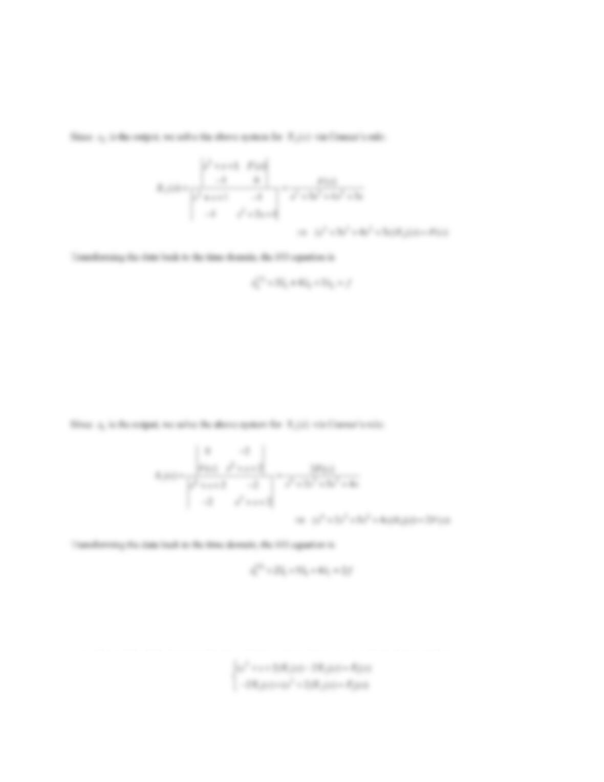
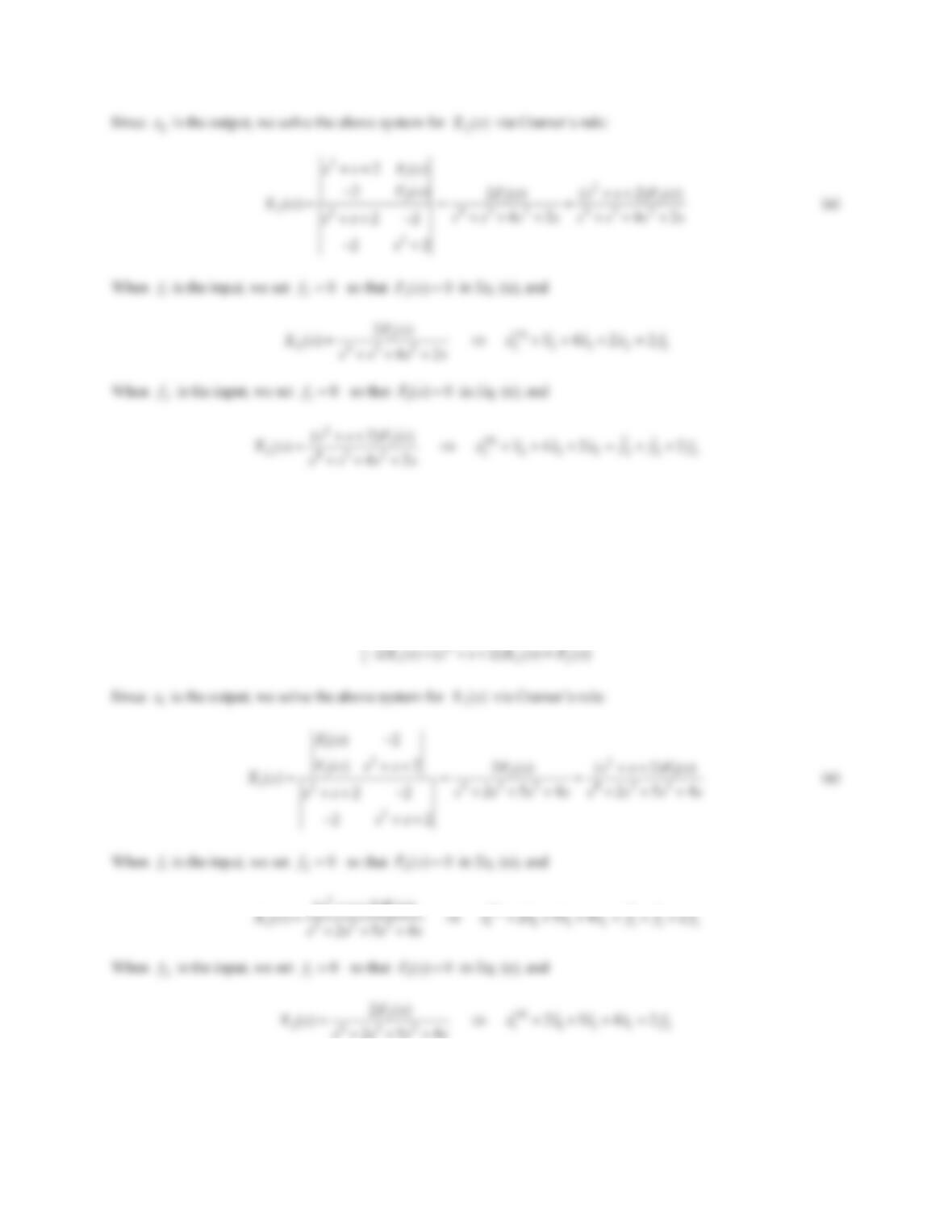
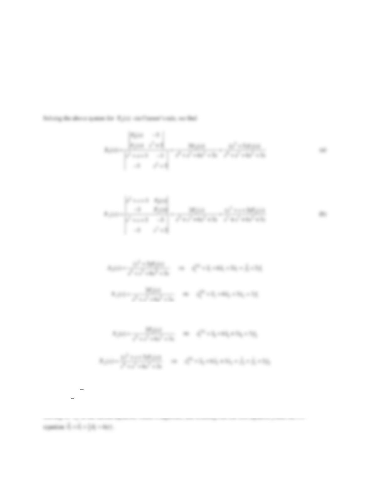
Solving the system for
2()Xs
via Cramer’s rule, we find
When
1
f
is the input, we set
2() 0Fs
in Eqns. (a) and (b), and two of the I/O equations are obtained as
When
2
f
is the input, we set
1
() 0Fs
in Eqns. (a) and (b), and the other two I/O equations are obtained as
6.
1
11 12
2
1
212
2
( ) ( )
( )
ht
TT TT
TTT
°
®
°
¯
,
()ht
=input,
1
T
=output
Solution
Solving for 2
in the second equation, which is algebraic, and inserting into the first equation yields the I/O
80
7.
1
11 12 1
2
212
2( ) ( )
2( )
qq qq q vt
qqq
°
®
°
¯
,
()vt
=input,
1
q
,2
q=outputs
Solution
There are two input-output equations. Proceeding as always,
2512
2
12
()()2()()
2 ( ) ( 2) ( ) 0
ss Qs QsVs
Qs s Q s
°
®
°
¯
8.
1
113 21 21
2
1
221 21
2
313
()()()
( ) 0
xxx x x x x ut
xxx xx
xxx
°
®
°
¯
,
()ut
=input,
1
x
,3
x=outputs
Solution
Two input-output equations are expected. Laplace transformation of the original system leads to
231
123
22
2
11
12
22
( ) () ( ) () () ()
( ) ( ) ( ) ( ) 0
ss Xs s XsXsUs
sXsssXs
°
°
®
81
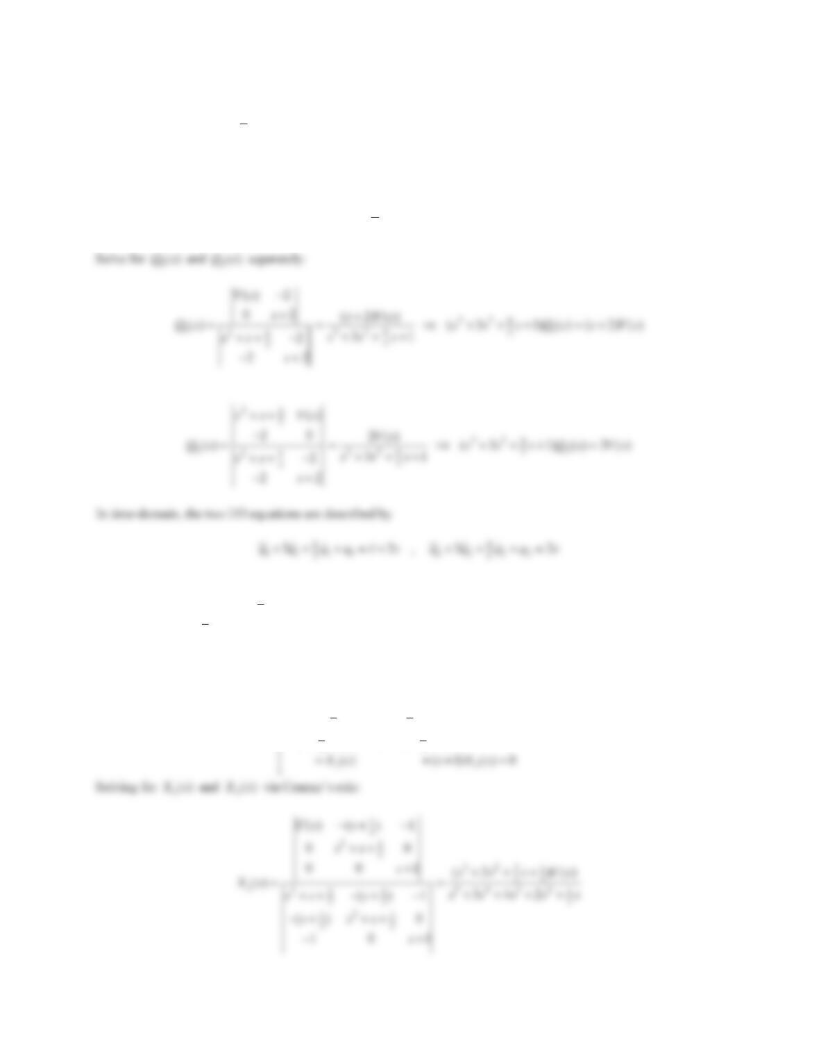
In time-domain, the two I/O equations are described by
9. Find the transfer matrix for the system described in Example 4.11.
Solution
Since there are two outputs and one input, the transfer matrix is
21u
in the form
10. Derive all possible input-output equations in Example 4.13.
Solution
The transfer matrix was obtained as
The four I/O equations are
(4)
1 111 111
1
235 2x x xxx fff
In Problems 11–14 the mathematical model of a system, as well as its inputs and outputs are provided. Find the
appropriate transfer matrix. Do not cancel any terms involving
s
in the numerator and denominator.
11.
1
11 12
3
11
22 21
23
( ) 0
()()
xx xx
xx xxft
°
®
°
¯
,()ft=input,
1
x
=output
Solution
Laplace transformation yields
82
211
12
33
2
111
12
323
( ) ( ) ( ) 0
() ( ) () ()
ss Xs Xs
Xs s s X s Fs
°
®
°
¯
Solving for
()Xs
results in
12.
1
11 12 1
2
1
212
2
() ()
( ) 0
qq qq q vt
qqq
°
®
°
¯
,
()vt
=input,
1
q
=output
Solution
Laplace transformation of the original system leads to
231
12
22
11
12
22
( ) () () ()
( ) ( ) ( ) 0
ss Qs QsVs
Qs s Q s
°
®
°
¯
13.
113 21 1
2212
313
2( ) ( )
2( ) ( )
xxx x x ft
xxxft
xxx
°
®
°
¯
,
1()ft
,2()ft
=inputs, 2
x,3
x=outputs
Solution
Taking the Laplace transform, we find
83
2
1231
(21)()2() ()()
ssXssXsXsFs
Solving separately for
2
()Xs
and
3()Xs
, yields
2
1
2
21 () 1
2()0
ss Fs
sFs
Note that we do not cancel terms involving
s
from the numerator and denominator in each fraction because
valuable information about the system will be lost otherwise. The entries of the
22u
transfer matrix
()sG
are
finally formed as
2 1
232
22
11 12
5432 5432
12
00
() ()
22 33
( ) , ( )
() ()
552 552
FF
Xs Xs
ss sss
Gs Gs
Fs F s
ssss ssss
14.
11 1 2 1
2122
2( ) ( )
2( ) ( )
xx xx ft
xxxft
®
¯
,
1()ft
,2()ft
=inputs,
1
x
,2
x=outputs
Solution
Laplace transformation of the original system leads to
84
We do not cancel terms involving
s
in the numerator and denominator in each fraction because valuable
information about the system may be lost otherwise. The entries of the
22u
transfer matrix
()sG
are formed as
2 1
2
11
11 12
43 2 43 2
12
00
() ()
22
( ) , ( )
() ()
42 42
FF
Xs Xs
s
Gs Gs
Fs F s
ss s s ss s s
15. A mechanical system model is derived as
()mx bx kx f t
where
1
3
m
,
2b
,
3k
, and applied force
1
2
() sin2ft t
, all in consistent physical units. Assuming
x
is the output, find the transfer function.
Solution
The transfer function is independent of the specific nature of the input, and is found as
16. In Problem 15 find the transfer function if x
is the output.
Solution
The transfer function is independent of the specific nature of the input. It is readily seen that
17. The governing equation for an electric circuit is
0
1() ()
t
di
LRi itdtvt
dt C
³
where
L
,
R
, and
C
are the
inductance, resistance, and capacitance, all constants,
()it
is the current and
()vt
is the applied voltage.
Assuming
()it
and
()vt
are the system output and input, respectively, find the transfer function.


