154
Rearranging the equations, we have
11 11 1 2 1 2 2 1
()mx bx k k x k x f
22 21 2 3 2 2
()mx kx k k x f
b. The differential equations can be expressed in second-order matrix form as
c. The state, the input, and the output are
11
xx
½½
The state-space representation in matrix form is
11
0010 00
0001 00
xx
ªº
ªº
«»
«»
½ ½
«»
«»
1
x
½
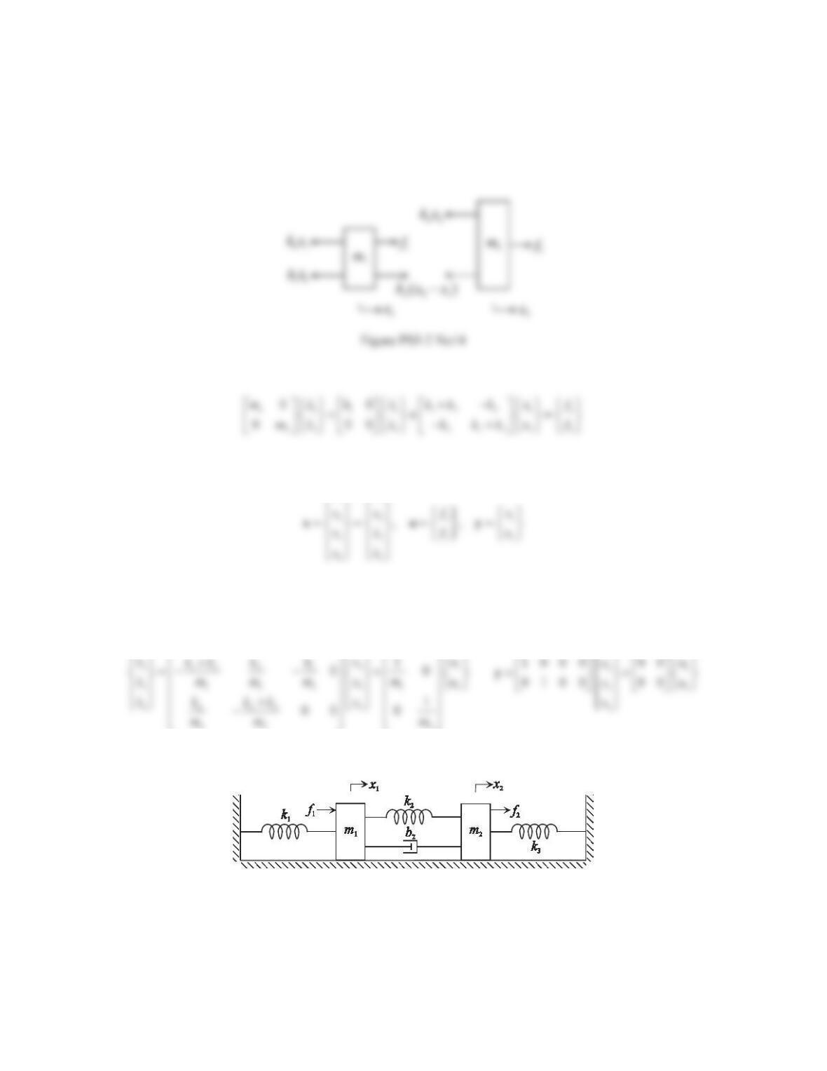
15. Repeat Problem 14 for the system shown in Figure 5.50.
Figure 5.50 Problem 15.
Solution
a. We choose the displacements of the two masses
1
x
and 2
xas the generalized coordinates. The static
equilibrium positions of
1
m
and
2
m
are set as the coordinate origins. Assume that
21
0xx!!
.
155
Figure PS5-2 No15
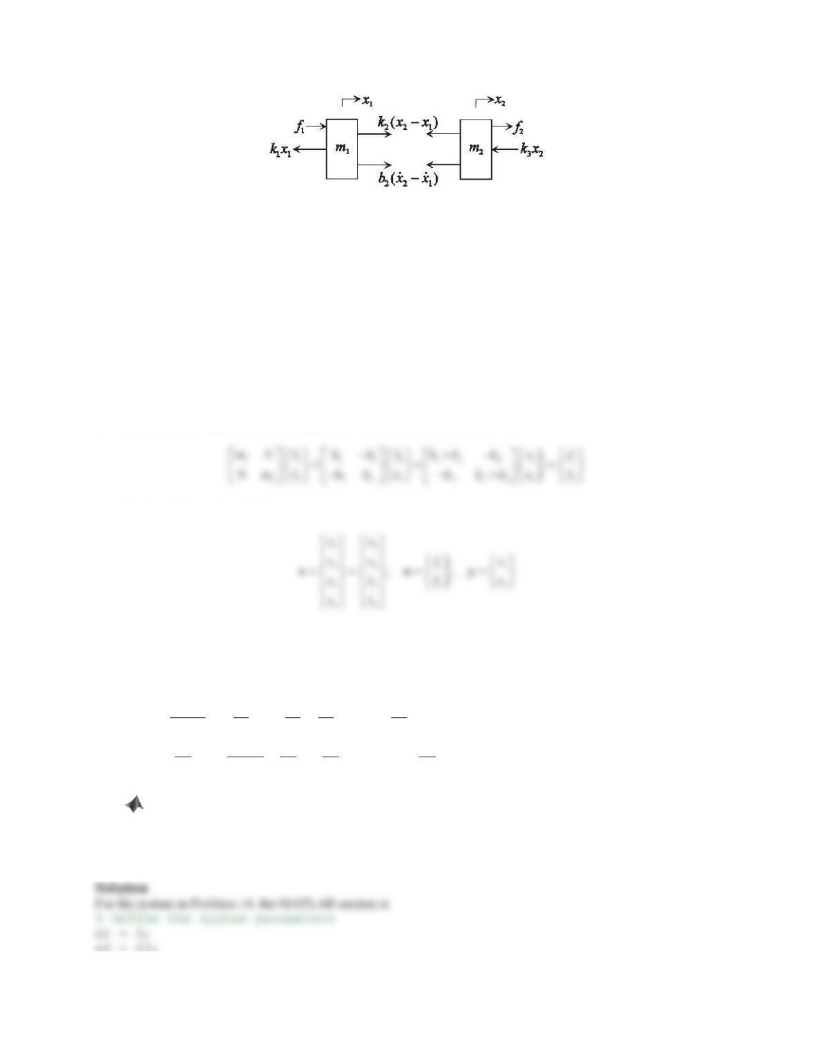
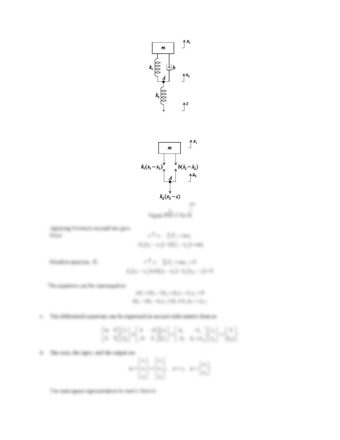
Applying Newton’s second law in the x-direction gives
:
xx
xFmao ¦
Mass 1:
11122 1 22 1 11
()()fkxkxx bxx mx
Mass 2:
2221 221 32 22
()()fkxx bxx kxmx
Rearranging the equations, we have
11 21 2 2 1 2 1 2 2 1
()mx bx bx k k x kx f
22 21 2 3 2 21 22 2
()mx kx k k x bx bx f
b. The differential equations can be expressed in second-order matrix form as
c. The state, the input, and the output are
The state-space representation in matrix form is
11
221
12 2 2 2
1111 1
332
44
23
222
2
2222
0010 00
0001 00
10
1
0
xx
xxu
kk k b b
mmmm m
xxu
xx
kk
kbb
m
mmmm
ªº
ªº
«»
«»
½ ½
«»
«»
°° °°
«»
«»
½
°° °°
®¾ ®¾ ®¾
«»
«»
¯¿
°° °°
«»
«»
°° °°
«»
«»
¯¿ ¯¿
«»
«»
¬¼
¬¼
,
1
21
32
4
1000 00
0100 00
x
xu
xu
x
½
°° ½
ªºªº
°°
®¾ ®¾
«»«»
¬¼¬¼¯¿
°°
°°
¯¿
y
16. For Problems 14 and 15, use MATLAB commands to define the systems in the state-space form and then
convert to the transfer function form. Assume that the displacements of the two masses, x1and x2, are the
outputs, and all initial conditions are zero. The masses are m1= 5 kg and m2= 15 kg. The spring constants are k1
= 7.5 kN/m, k2= 15 kN/m, and k3= 30 kN/m. The viscous damping coefficients are b1= 280 N·s/m and b2= 90
N·s/m.
156
The command tf returns four transfer functions
1
2
1
2
12
0.2 600 200
() ()
() () 200 0.06667 3.733 300
s
Xs Xs
Fs F s ss
ªº
ªº
«»
«»
«»
¬¼
The command tf returns four transfer functions for the system in Problem 15
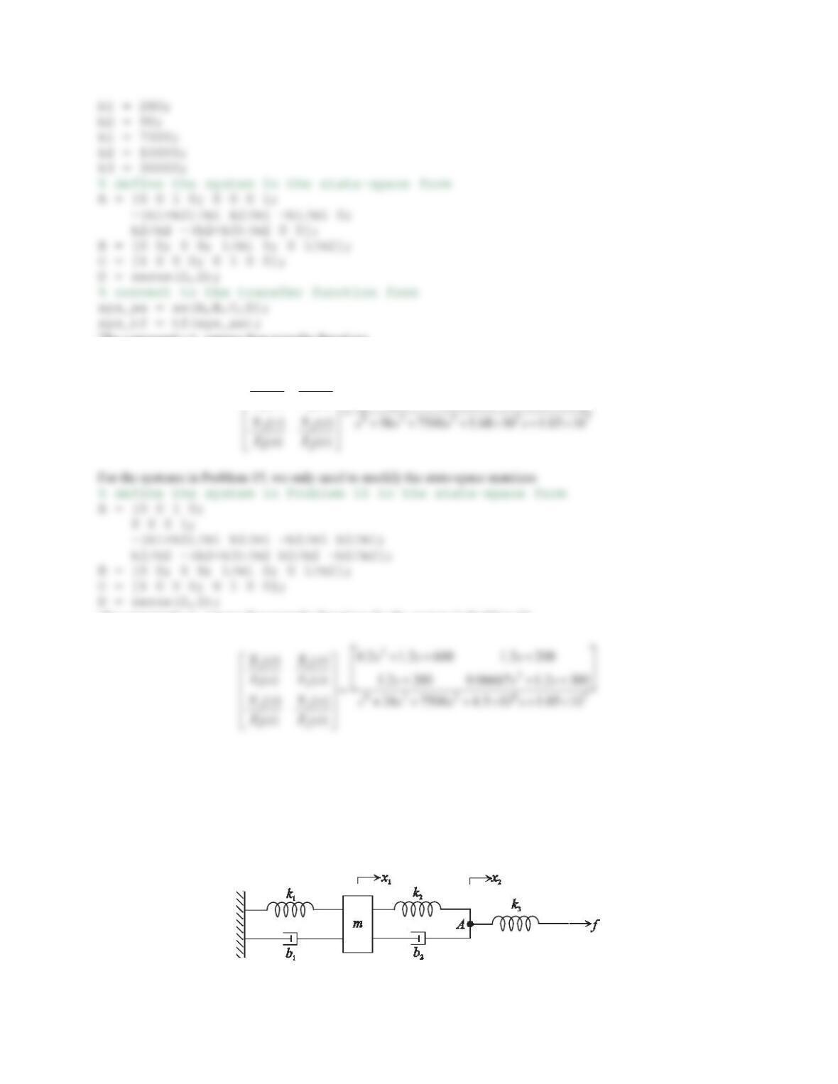
17. For the system in Figure 5.51, the input is the force fand the outputs are the displacement x1of the mass and the
displacement x2of the massless junction A.
a. Draw the necessary free-body diagrams and derive the differential equations of motion. Determine the
number of degrees of freedom and the order of the system.
b. Write the differential equations of motion in the second-order matrix form.
c. Using the differential equation obtained in Part (a), determine the state-space representation.
Figure 5.51 Problem 17.
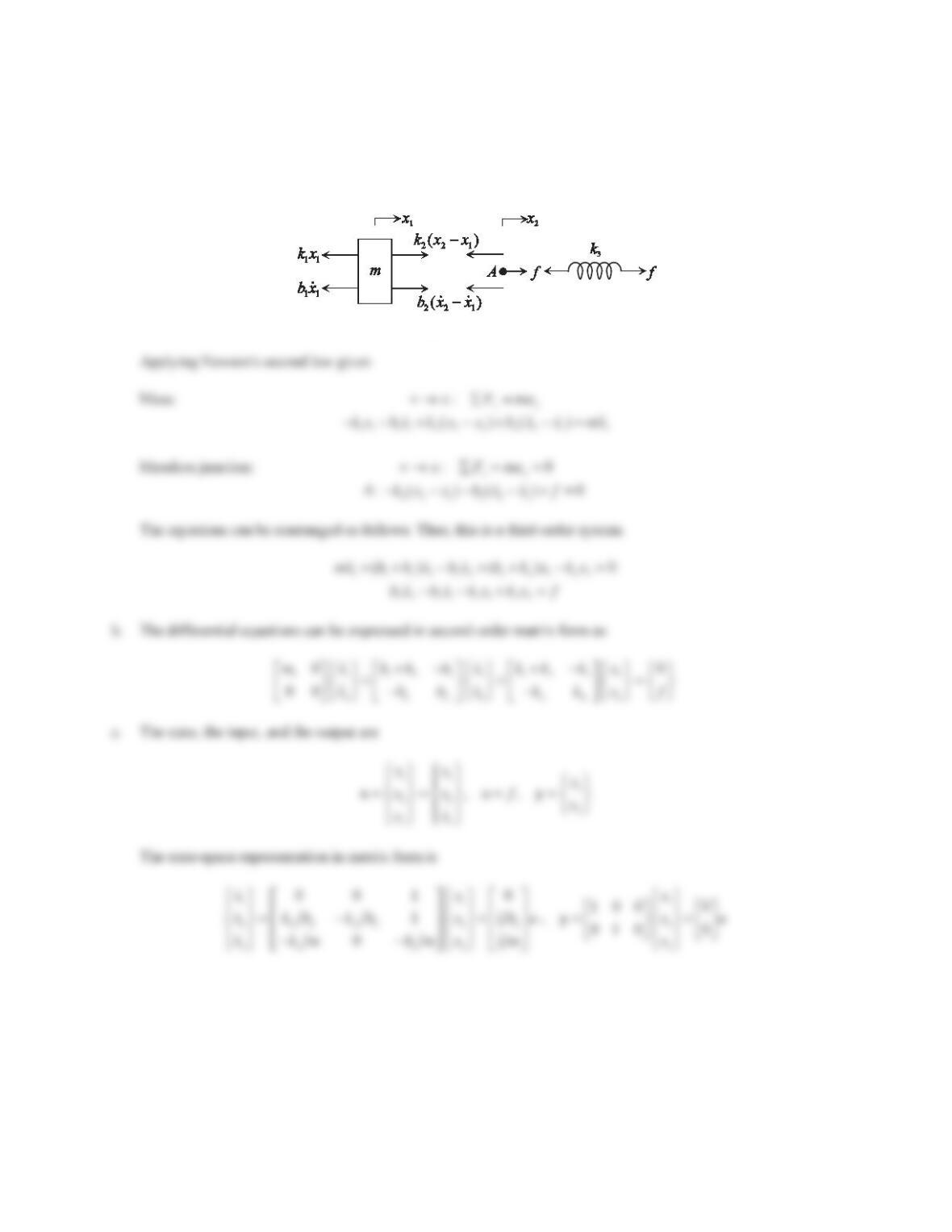
157
Solution
a. One massless junction is included in this system. We choose the displacements of the mass and the junction A
as the generalized coordinates, which are denoted by
1
x
and 2
x. Thus, this is a two-degree-of-freedom system.
Assume that
21
0xx!!
.
Figure PS5-2 No17
18. Repeat Problem 17 for the system in Figure 5.52, the input is the displacement zand the outputs are the
displacements x1and x2.
158
Figure 5.52 Problem 18.
Solution
a. Assume that
12
0xxz!!!
.
b.
159
Problem Set 5.3
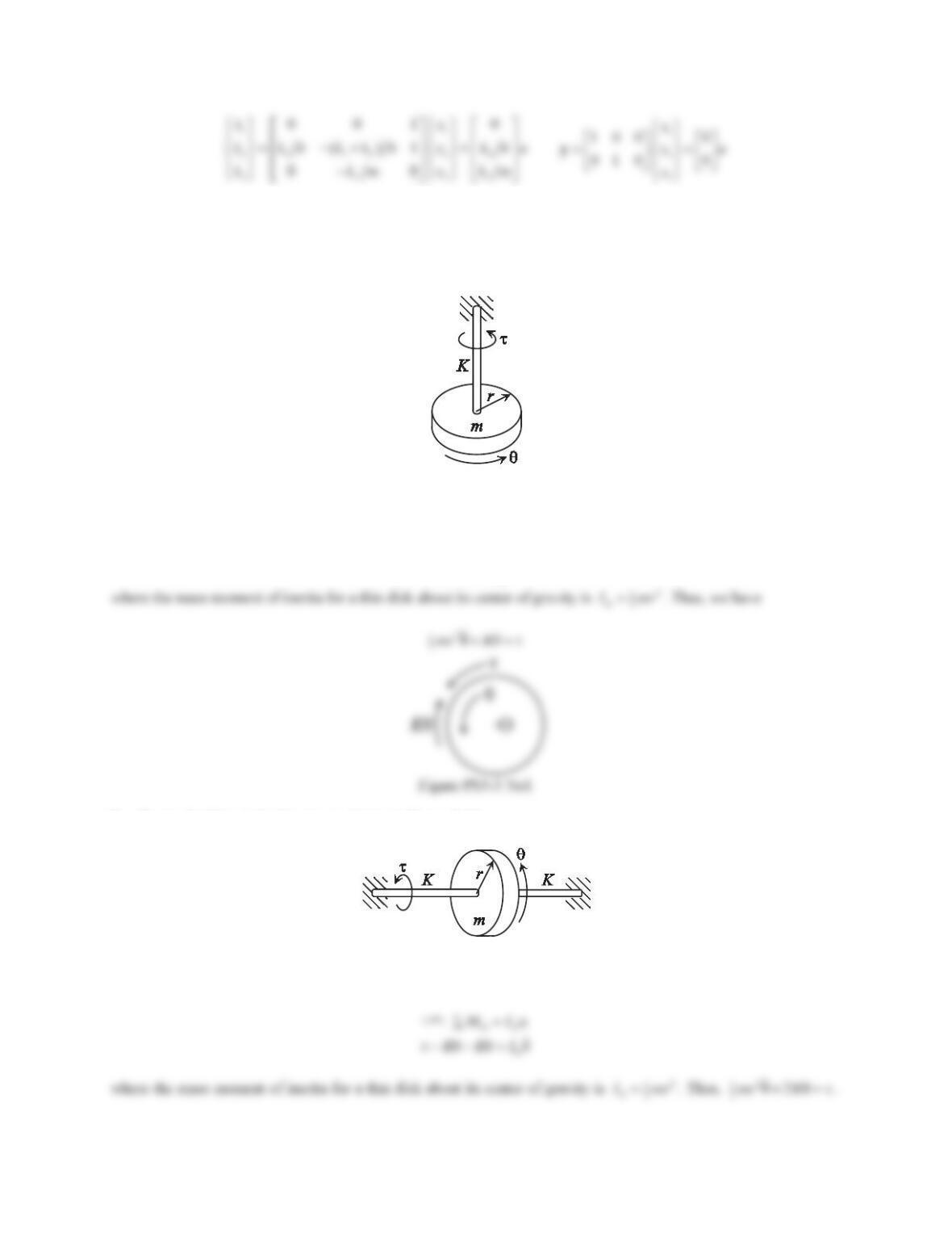
1. Consider the rotational system shown in Figure 5.61. The system consists of a massless shaft and a uniform thin
disk of mass mand radius r. The disk is constrained to rotate about a fixed longitudinal axis along the shaft. The
shaft is equivalent to a torsional spring of stiffness K. Draw the necessary free-body diagram and derive the
differential equation of motion.
Figure 5.61 Problem 1.
Solution
The free-body diagram of the disk is shown below. Applying the moment equation to the fixed point O gives
+ր:
OO
ĮMI¦
O
IJș șKI
2. Repeat Problem 1 for the system shown in Figure 5.62.
Figure 5.62 Problem 2.
Solution
The free-body diagram of the disk is shown below. Applying the moment equation to the fixed point O gives
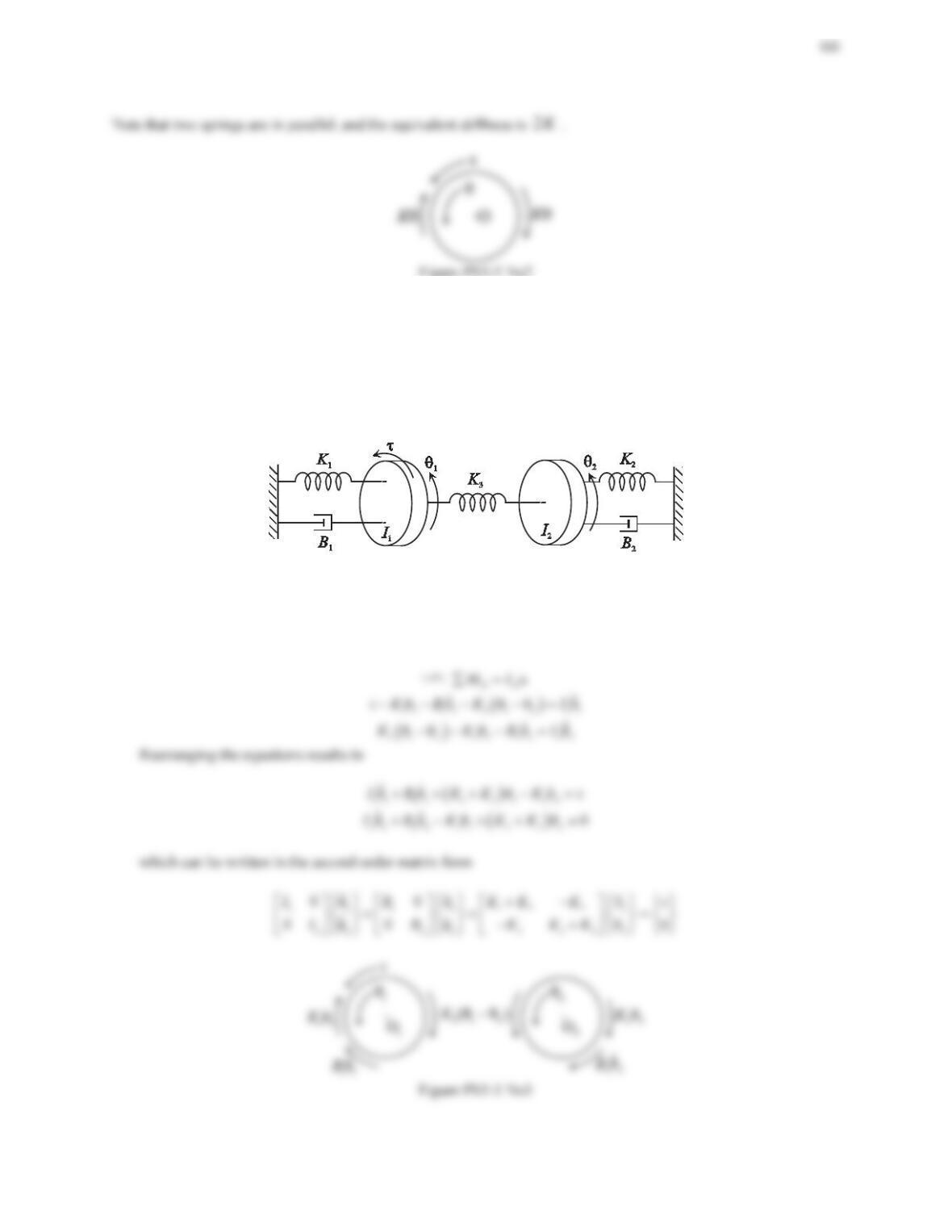
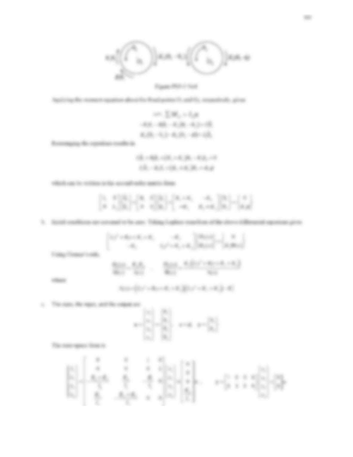
3. Consider the torsional mass–spring–damper system in Figure 5.63. The mass moments of inertia of the two
disks about their longitudinal axes are I1and I2, respectively. The massless torsional springs represent the
elasticity of the shafts and the torsional viscous dampers represent the fluid coupling.
a. Draw the necessary free-body diagrams and derive the differential equations of motion. Provide the
equations in the second-order matrix form.
b. ‘HWHUPLQHWKHWUDQVIHUIXQFWLRQVĬ1(s)/T(sDQGĬ2(s)/T(s). All the initial conditions are assumed to be zero.
c. Determine the state–VSDFHUHSUHVHQWDWLRQZLWKWKHDQJXODUGLVSODFHPHQWVș1DQGș2as the outputs.
Figure 5.63 Problem 3.
Solution
a. We choose the angular displacements T1and T2as the generalized coordinates. Assume that 12
șș!!
. The
free-body diagrams are shown in the figure below. Applying the moment equation about the fixed points O1and
O2, respectively, gives
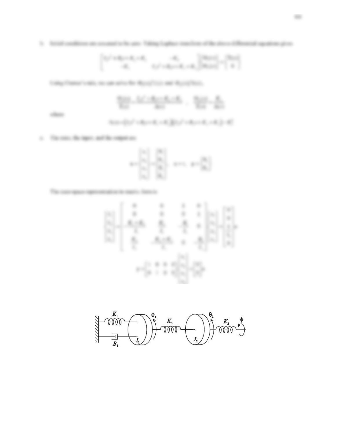
4. Repeat Problem 3 for the system shown in Figure 5.64. The input is the angular displacement Iat the end of the
shaft.
Figure 5.64 Problem 4.
Solution
a. Assume that
12
șș
I
!!!
. The free-body diagrams are shown in the figure below.
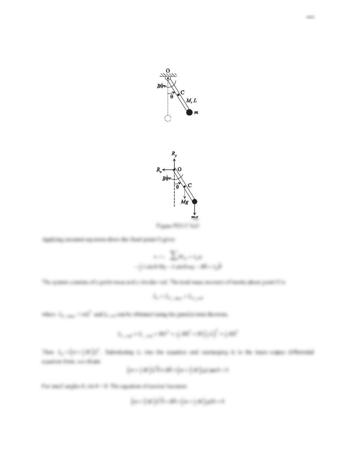
5. Consider the pendulum system shown in Figure 5.65. The system consists of a bob of mass mand a uniform rod
of mass Mand length L. The pendulum pivots at the joint O. Draw the necessary free-body diagram and derive
WKHGLIIHUHQWLDOHTXDWLRQRIPRWLRQ$VVXPHVPDOODQJOHVIRUș
Figure 5.65 Problem 5.
Solution
For the pendulum system, the free-body diagram is shown below, where Rxand Ryare the xand ycomponents of the
reaction force at the joint O, respectively. Note that the system rotates about a fixed axis through the point O.
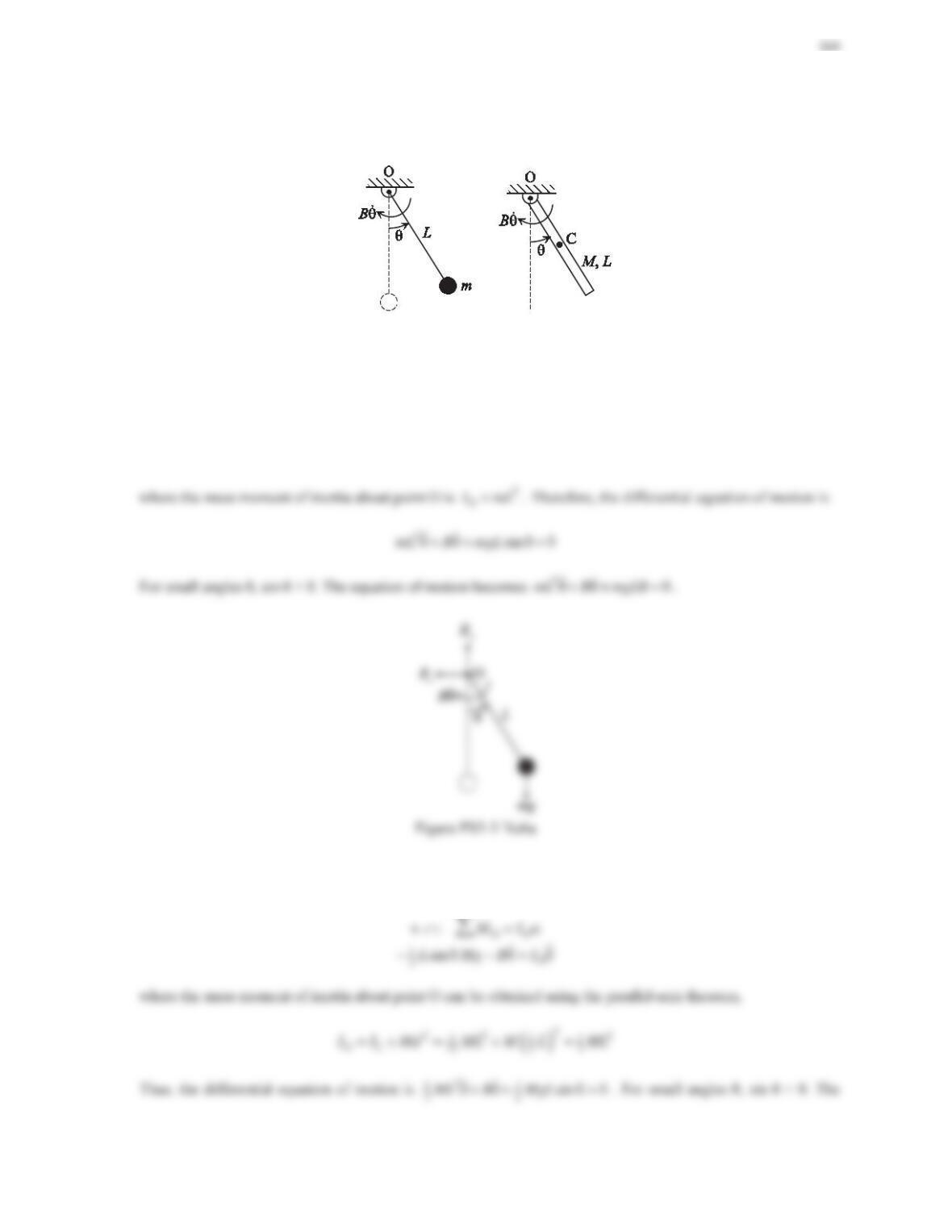
6. Repeat Problem 5 for the systems shown in Figure 5.66, where (a) the mass of the rod is neglected and (b) no
bob is attached to the rod.
(a) (b)
Figure 5.66 Problem 6.
Solution
a. The free-body diagram of the system in (a) is shown below, where the mass of the rod is neglected. Applying
moment equation about the fixed point O gives
OO
:MI D
¦
{
O
sin ·LmgBITT T
b. The free-body diagram of the system in (b) is shown below, where no bob is attached to the rod. Applying
moment equation about the fixed point O gives
165
equation of motion becomes
2
11
32
0ML B MgLT T T
.
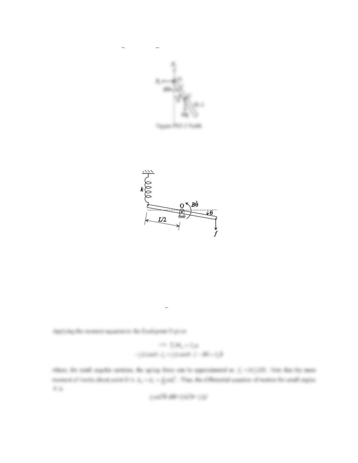
7. The system shown in Figure 5.67 consists of a uniform rod of mass mand length Land a translational spring of
stiffness kat the rod’s left tip. The friction at the joint O is modeled as a damper with coefficient of torsional
viscous damping B. The input is the force fDQGWKHRXWSXWLVWKHDQJOHș7KHSRVLWLRQș FRUUHVSRQGVWRWKH
static equilibrium position when f= 0.
Figure 5.67 Problem 7.
a. Draw the necessary free-ERG\GLDJUDPDQGGHULYHWKHGLIIHUHQWLDOHTXDWLRQRIPRWLRQIRUVPDOODQJOHVș
b. Using the linearized differential equation obtained in Part (a GHWHUPLQH WKH WUDQVIHU IXQFWLRQ Ĭs)/F(s).
Assume that the initial coQGLWLRQVDUHș DQG
ș
.
c. Using the differential equation obtained in Part (a), determine the state-space representation.
Solution
a. At equilibrium, we have
+ց:
O
0M¦
1
st
20Lk
G
st 0
G

166
Figure PS5-3 No7
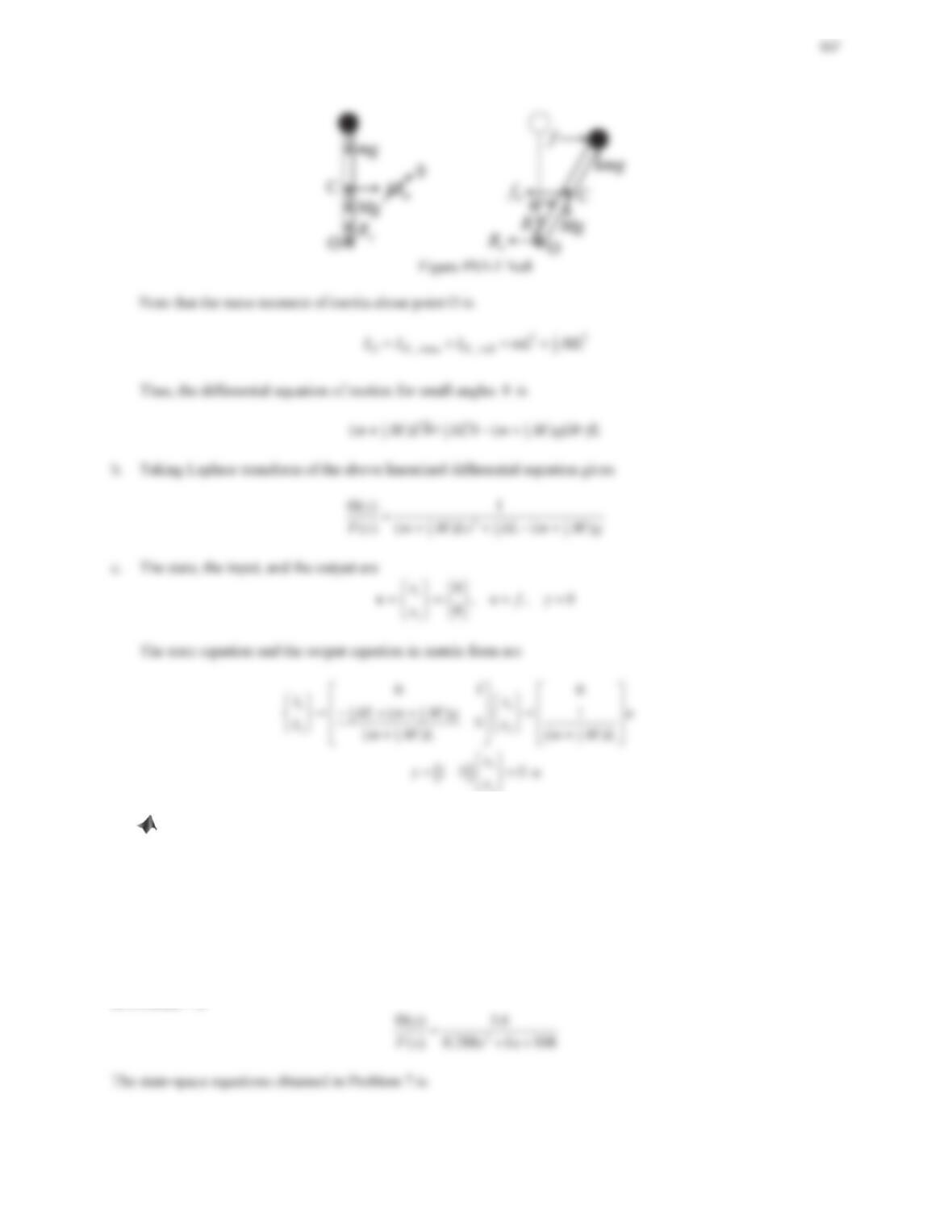
b. Taking Laplace transform of the above linearized differential equation gives
22 2
() 6
( ) 12 3
sL
Fs mLs Bs kL
4
c. The state, the input, and the output are
1
2
ș,,ș
ș
xuf y
x
½½
®¾®¾
¯¿
¯¿
x
The state equation and the output equation in matrix form are
11
22
2
01 0
312 6
xx
u
kB
xx
mmL mL
ªºªº
½ ½
«»«»
®¾ ®¾
«»«»
¯¿ ¯¿
¬¼¬¼
,
>@
1
2
10 0
x
yu
x
½
®¾
¯¿
8. Repeat Problem 7 for the system shown in Figure 5.68. 7KHSRVLWLRQș FRUUHVSRQGVWRWKHstatic equilibrium
position when f= 0.
Figure 5.68 Problem 8.
Solution
a. At equilibrium, we have
+ց:
O
0M¦
1
st
20Lk
G
st 0
G
9. Example 5.4 Part (d) shows how one can represent a linear system in Simulink based on the differential
equation of the system. A linear system can also be represented in transfer function or state-space form. The
corresponding blocks in Simulink are Transfer Fcn and State-Space, respectively. Refer to Problem 7.
&RQVWUXFW D 6LPXOLQN EORFN GLDJUDP WR ILQG WKH RXWSXW șt) of the system, which is represented using (a) the
linearized differential equation of motion, (b) the transfer function, and (c) the state-space form obtained in
Problem 7. The parameter values are m= 0.8 kg, L= 0.6 m, k= 100 N/m, B= 0.5 N·s/m, and g= 9.81 m/s2.The
input force fis the unit-impulse function, which has a magnitude of 10 N and a time duration of 0.1 s.
Solution
The linearized equation of motion obtained in Problem 7 is
0.024șșș f
. The transfer function obtained
in Problem 7 is
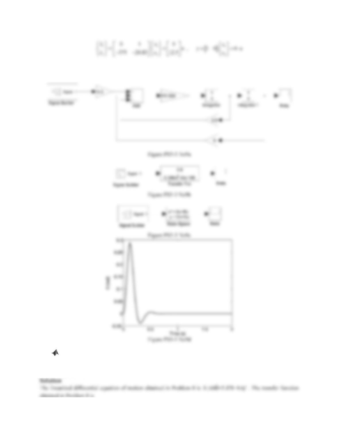
168
The Simulink block diagrams constructed based on the differential equation, the transfer function, the state-space
form are shown below. Run simulations and the same response in Plot d is obtained.
10. Repeat Problem 9 using the linearized differential equation of motion, the transfer function, and the state–
space form obtained in Problem 8. The parameter values are m= 0.2 kg, M= 0.8 kg, L= 0.6 m, k= 100 N/m,
and g= 9.81 m/s2. The input force fis the unit-impulse function, which has a magnitude of 10 N and a time
duration of 0.1 s.
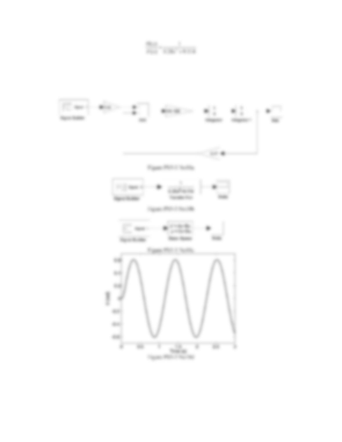
169
The state-space equations obtained in Problem 7 is
11
22
01 0
32.55 0 3.57
xx
u
xx
½ ½
ªºªº
®¾ ®¾
«»«»
¯¿¬ ¼¯¿¬ ¼
,
>@
1
2
10 0
x
yu
x
½
®¾
¯¿
11. Consider the system shown in Figure 5.69, where the motion of the rod is small angular rotation. When ș ,
the springs are at their free lengths.
a. Determine the mass moment of inertia of the rod about point O. Assume that a>b.
b. Draw the necessary free-body diagram and derive the differential equation of motion for small angles T.
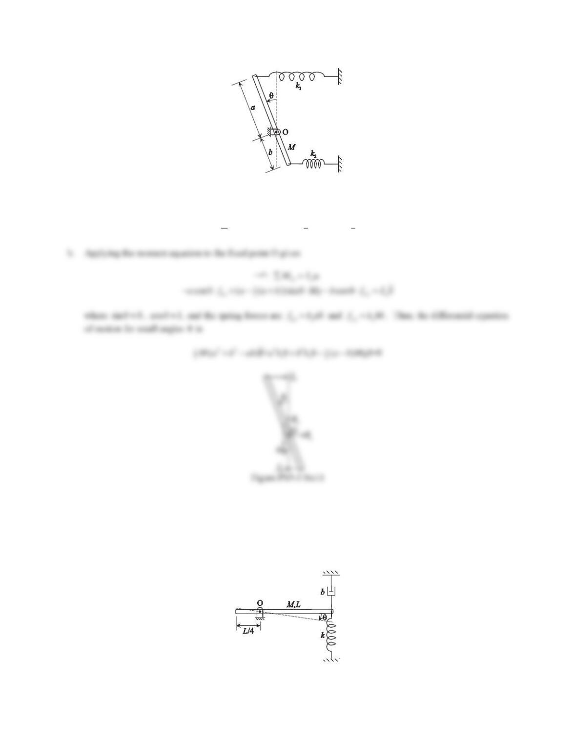
170
Figure 5.69 Problem 11.
Solution
a. Applying the parallel axis theorem gives the mass moment of inertia of the rod about point O
2
22 22
111
OC 12 2 3
() () ( )IIMd MabMa ab Mabab
12. Consider the system shown in Figure 5.70, where a lever arm has a spring–damper combination on the other
side. When ș , the system is in static equilibrium.
a. Assuming that the lever arm can be approximated as a uniform slender rod, determine the mass moment of
inertia of the rod about point O.
b. Draw the necessary free-body diagram and derive the differential equation of motion for small angles T.
Figure 5.70 Problem 12.
171
Solution
a. Applying the parallel axis theorem gives the mass moment of inertia of the rod about point O
2
22 2
7
111
OC 12 2 4 48
I I Md ML M L L ML
b. At equilibrium, we have
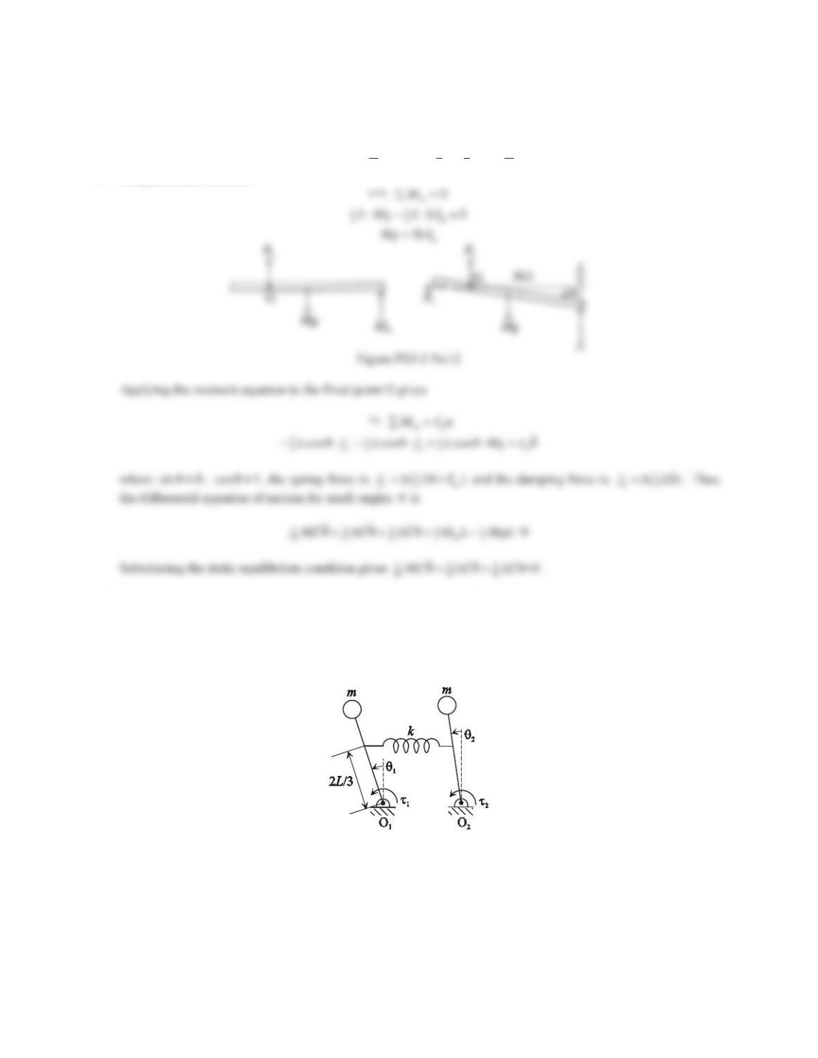
13. Consider the two-degree-of-freedom system shown in Figure 5.71, where two simple inverted pendulums are
connected by a translational spring of stiffness k. Each pendulum consists of a point mass mconcentrated at the
tip of a massless rod of length L7KHLQSXWVDUHWKHWRUTXHVIJ1DQGIJ2applied to the pivot points O1and O2,
UHVSHFWLYHO\7KHRXWSXWVDUHWKHDQJXODUGLVSODFHPHQWVș1DQGș2RIWKHSHQGXOXPV:KHQș1 ș2 IJ1= 0,
DQGIJ2= 0, the spring is at its free length.
Figure 5.71 Problem 13.
a. Draw the necessary free-body diagrams and derive the differential equations of motion. Assume small
DQJOHVIRUș1DQGș2. Provide the equations in the second-order matrix form.
b. Using the differential equations obtained in Part (a), determine the state-space representation with the
angular velocities
1
T
and
2
T
as the outputs.
172
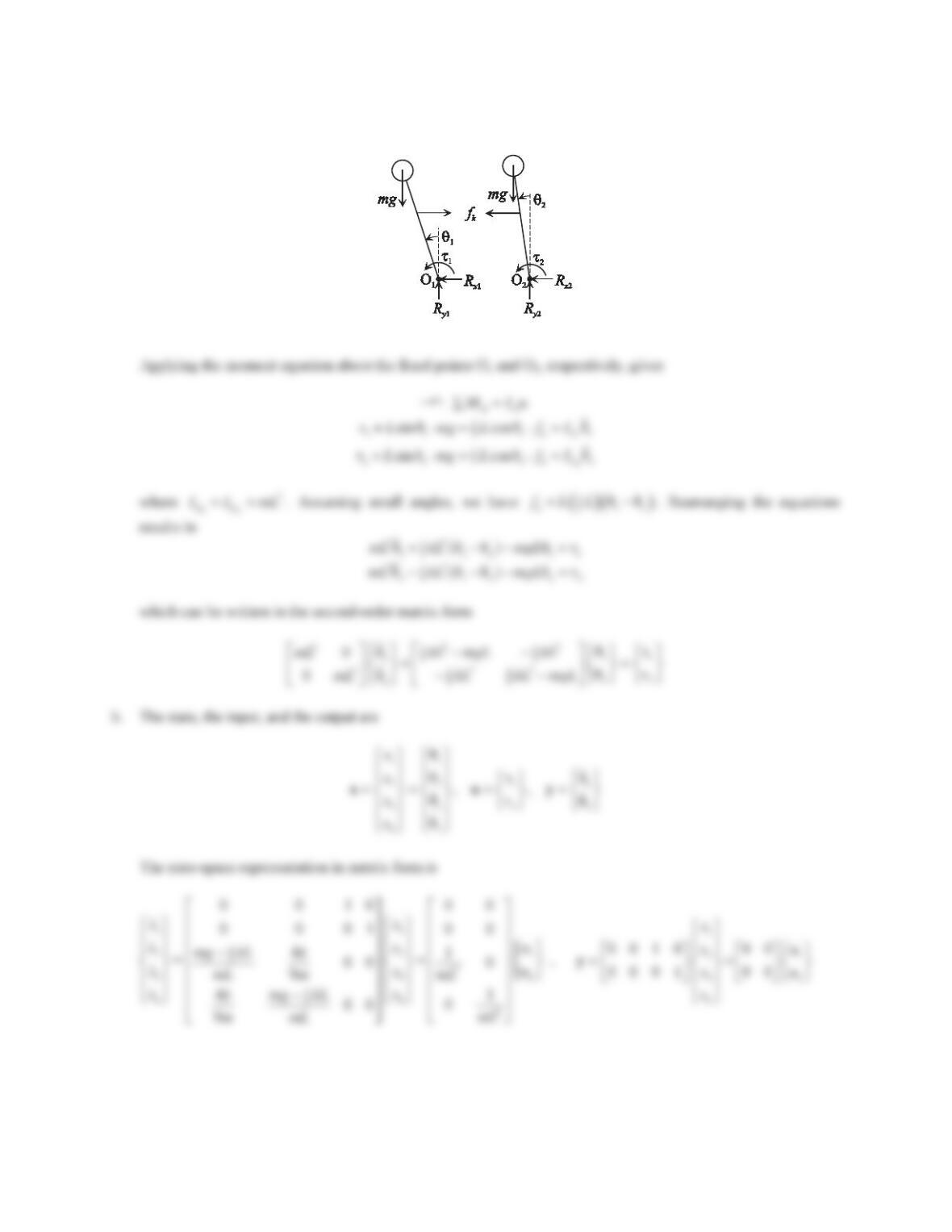
Solution
a. Assume that 12
șș!!
. The free-body diagrams are shown in the figure below.
Figure PS5-3 No13
14. Repeat Problem 13 for the system shown in Figure 5.72, where each pendulum is a uniform slender rod of mass
mand length L.
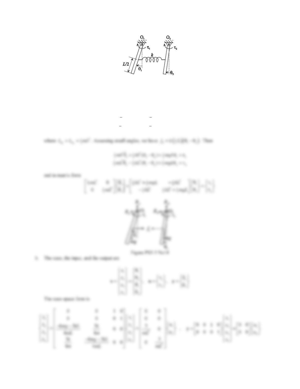
173
Figure 5.72 Problem 14.
Solution
a. Assume that 12
șș!!
. The free-body diagrams are shown in the figure below. Applying the moment equation
about the fixed points O1and O2, respectively, gives
+ց:
OO
ĮMI¦
1
11
11 1O1
22
IJVLQș FRVș ș
k
LmgL fI
2
11
22 2O2
22
IJVLQș FRVș ș
k
LmgL fI