242
Figure 6.38 Problem 2.
Solution
Because the current drawn by the op-amp is very small, i.e., 0ii
||
, we have at node 1,
12
ii
o
1
12
vv
vv
RR
or
21 1o 1 2
()Rv Rv R R v
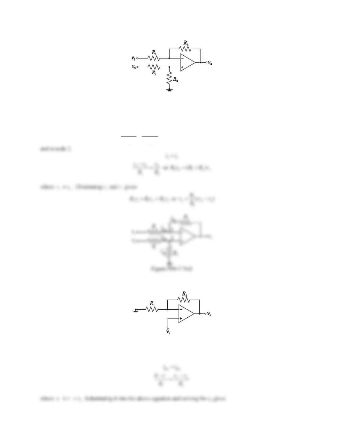
3. The op-amp circuit shown in Figure 6.39 is a non-inverting amplifier. Determine the relation between the input
voltage viand the output voltage vo.
Figure 6.39 Problem 3.
Solution
Because the current drawn by the op-amp is very small, i.e., 0ii
||
, we have
243
4. Consider the op-amp integrator circuit shown in Figure 6.35. Derive the differential equation relating the input
voltage viand the output voltage vo.
Solution
Note that the current drawn by the op-amp is very small. Applying Kirchhoff’s current law gives
RC
ii
i
o
vv d
Cvv
Rdt
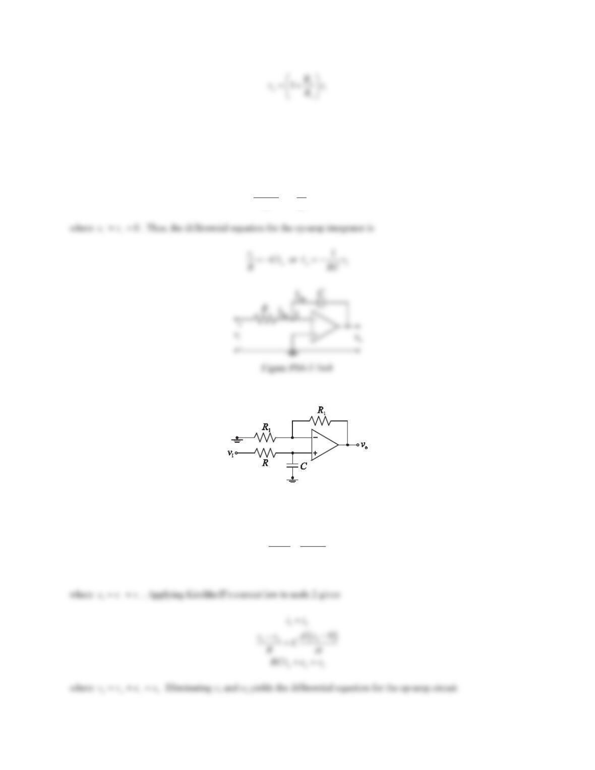
5. Consider the op-amp circuit shown in Figure 6.40. Derive the differential equation relating the input voltage vi
and the output voltage vo.
Figure 6.40 Problem 5.
Solution
Applying Kirchhoff’s current law to node 1 gives
12
ii
1o
1
11
0vv
v
RR
o1
2vv
244
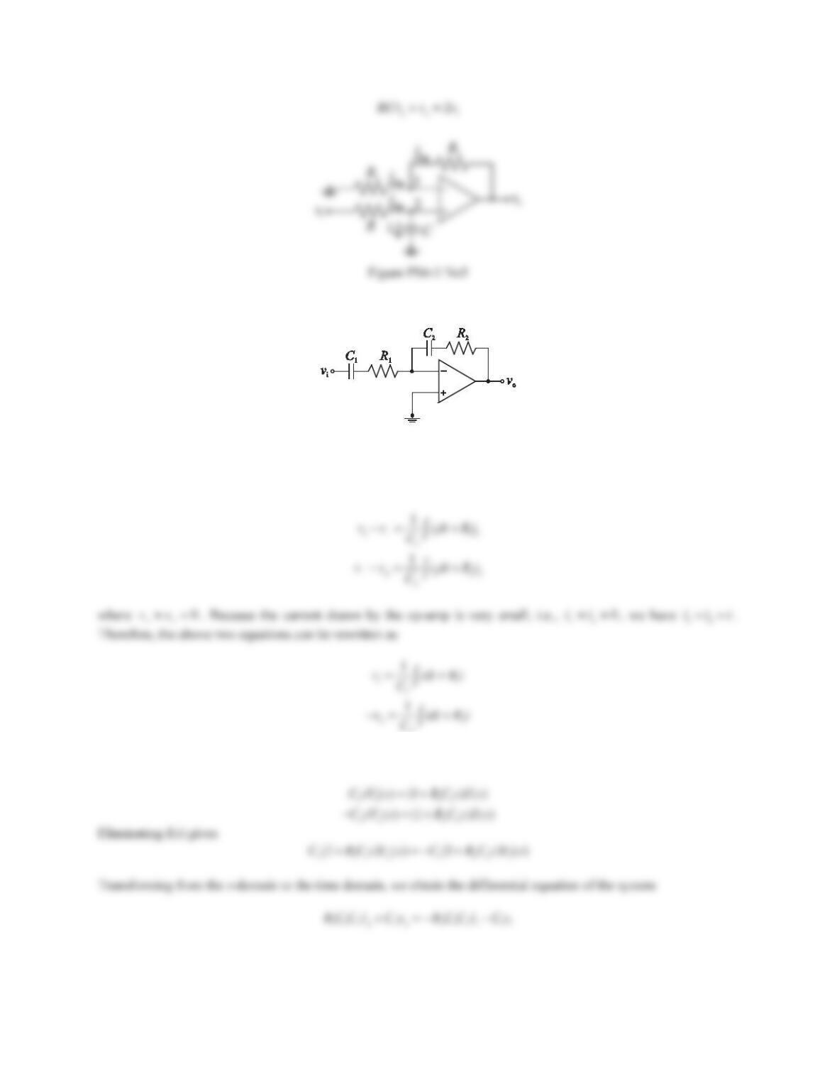
6. Repeat Problem 5 for the op-amp circuit shown in Figure 6.41.
Figure 6.41 Problem 6.
Solution
Denote the currents entering and leaving the node as i1and i2, respectively. We have
2
or in the s-domain with the assumption of zero initial conditions,
245
Problem Set 6.4
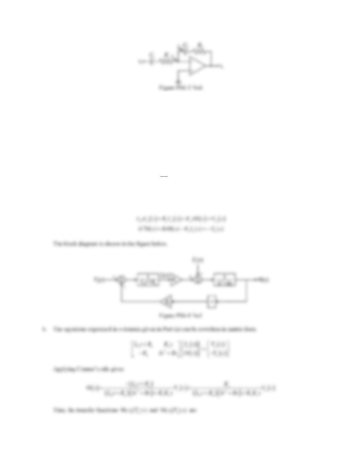
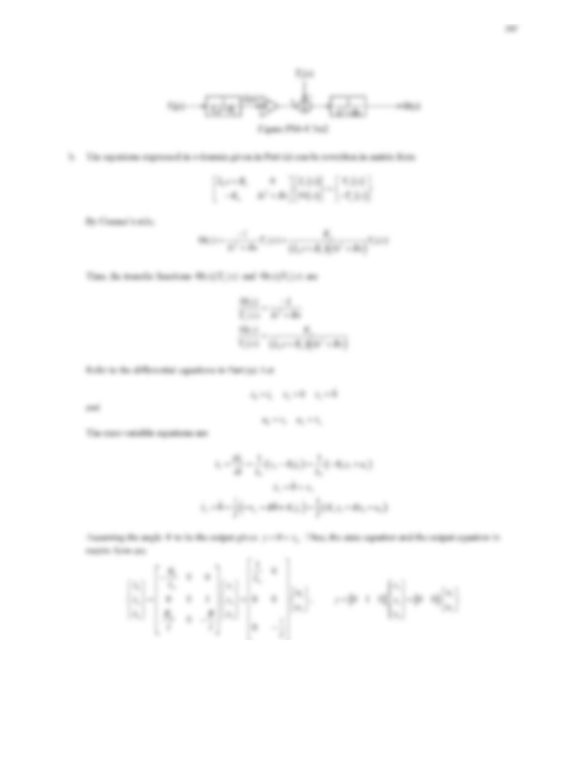
1. Reconsider the armature-controlled motor in Figure 6.44. Equations 6.31 and 6.32 represent the dynamics of the
system in terms of the variables iaand T.
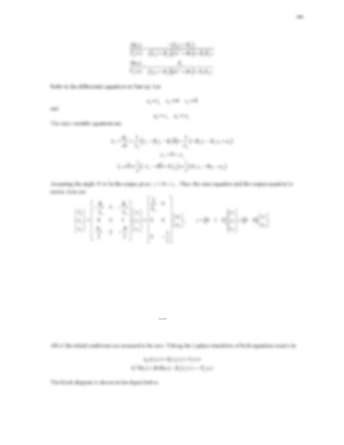
a. Assuming the angle șto be the output, draw a block diagram to represent the dynamics of the armature–
controlled motor.
b. Derive the transfer functions Ĭs)/Va(s)andĬs)/TL(s). All of the initial conditions are assumed to be zero.
Determine the state-space form.
Solution
a. Assuming the angle șto be the output, the differential equations of the system are
a
aaaea
ș
di
LRiKv
dt
ta L
șș IJIBKi
All of the initial conditions are assumed to be zero. Taking the Laplace transform of both equations results in
2. Reconsider the field-controlled motor in Figure 6.47. Equations 6.44 and 6.45 represent the dynamics of the
system in terms of the variables ifand T.
a. Assuming the angle șto be the output, draw a block diagram to represent the dynamics of the field–
controlled motor.
b. Derive the transfer functions Ĭs)/Vf(s)andĬs)/TL(s). All of the initial conditions are assumed to be zero.
Determine the state-space form.
Solution
a. The differential equations of the field-controlled DC motor shown in Figure 6.47 are
f
ffff
d
d
i
LRiv
t
tf L
șș IJIBKi
3. Consider the electromechanical system shown in Figure 6.49a. It consists of a cart of mass mmoving without
slipping on a ground track. The cart is equipped with an armature-controlled DC motor, which is coupled to a
rack and pinion mechanism to convert the rotational motion to translation and to create the driving force ffor
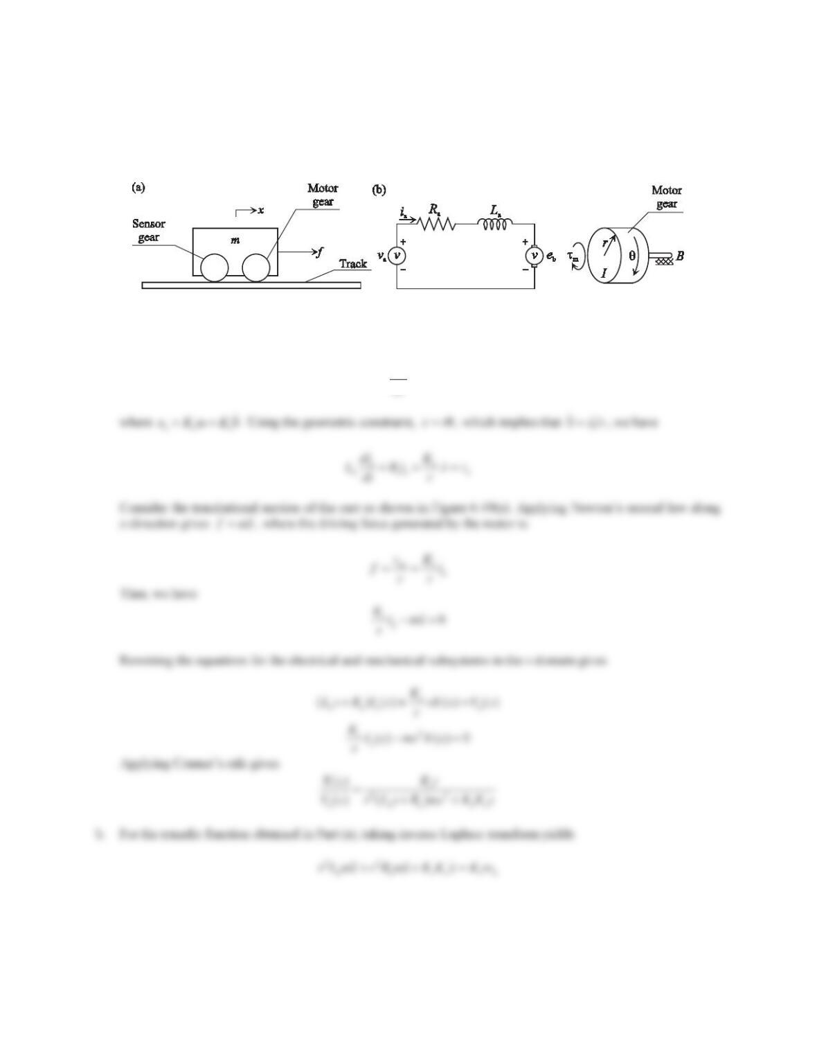
248
the system. Figure 6.49b shows the equivalent electric circuit and the mechanical model of the DC motor, where
ris the radius of the motor gear. The torque and the back emf constants of the motor are Ktand Ke, respectively.
a. Determine the transfer function X(s)/Va(s). Assume that all initial conditions are zero.
b. Determine the differential equation of the system relating the cart position xand the applied voltage va.
Figure 6.49 Problem 3.
Solution
a. For the electrical circuit shown in Figure 6.49(b), applying Kirchhoff’s voltage law gives
a
aa a b a 0
di
Ri L e v
dt
4. Consider the single-link robot arm as shown in Figure 6.50a. It is driven by an armature-controlled DC motor
through spur gears with a total gear ratio of N. The mass moments of inertia of the motor and the load are Imand
I, respectively. The coefficients of torsional viscous damping of the motor and the load are Bmand B,
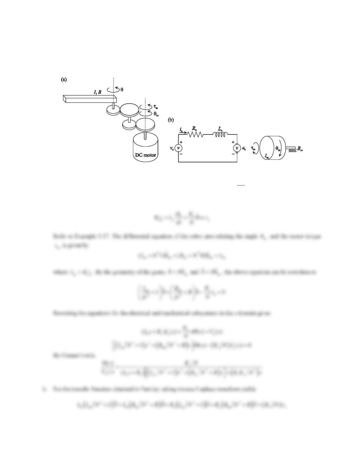
249
respectively. Figure 6.50b shows the equivalent electric circuit and the mechanical model of the DC motor. The
torque and the back emf constants of the motor are Ktand Ke, respectively.
a. Determine the transfer function Ĭs)/Va(s). Assume that all initial conditions are zero.
b. Determine the differential equation relating the applied voltage vaand the link angular displacement ș.
Figure 6.50 Problem 4.
Solution
a. The differential equation of the electrical subsystem of the motor is
a
aa a b a
0
di
Ri L e v
dt
where
bem
șeK
.
By the geometry of the gears, m
șșN
,where Nis the gear ratio, we have
250
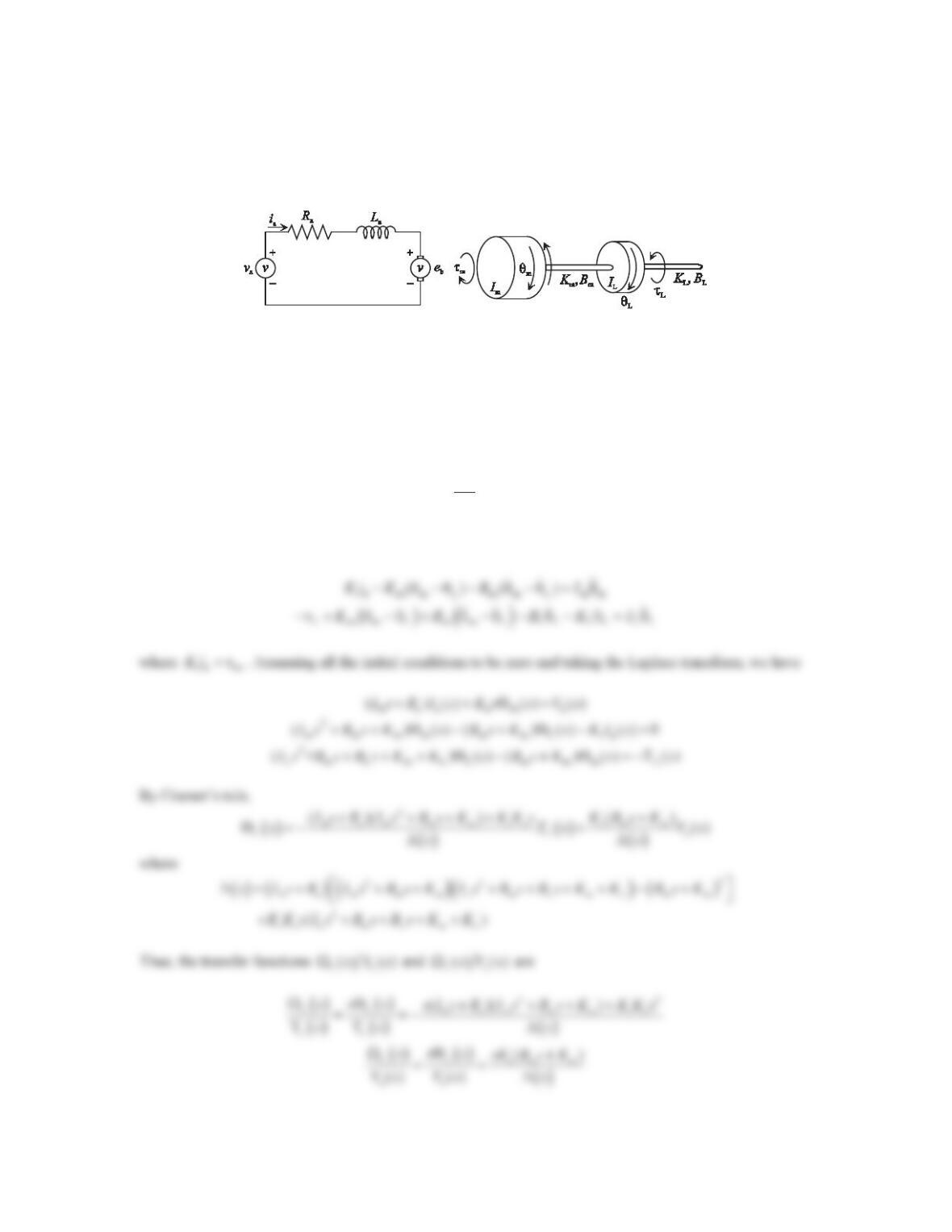
5. A more complicated model of the armature-controlled motor is shown in Figure 6.51, where the rotor is
connected to an inertial load through a flexible and damped shaft. Kmand Bmrepresent the torsional stiffness
and the torsional viscous damping of the shaft, respectively. The mass moments of inertia of the motor and the
load are Imand IL, respectively. Let
mm
Ȧș
and
LL
Ȧș
.
Figure 6.51 Problem 5.
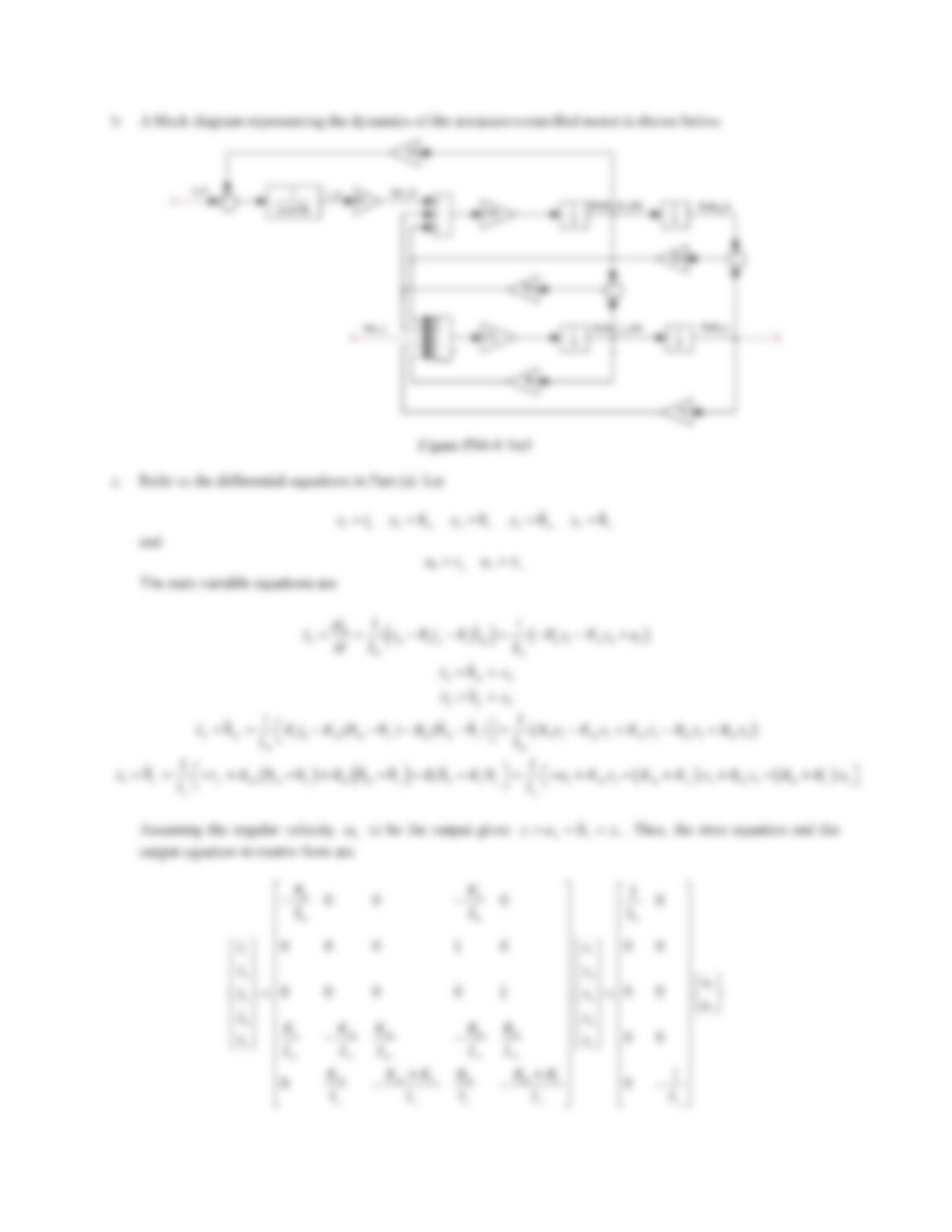
a. Derive the transfer functions ȍL(s)/Va(s)andȍL(s)/TL(s). Assume all of the initial conditions to be zero.
b. Assuming the angular velocity ȦLto be the output, draw a block diagram to represent the dynamics of the
armature-controlled motor.
c. Determine the state-space form assuming the angular velocity ȦLto be the output.
Solution
a. For the electrical part, applying Kirchhoff’s current law gives
a
aa a e m a
d
dș
i
Ri L K v
t
where
em b
șKe
. The mechanical part becomes a two-degree-of-freedom system. Assuming that șm>șLand
applying the moment equation to the rotor and the load gives
251
252
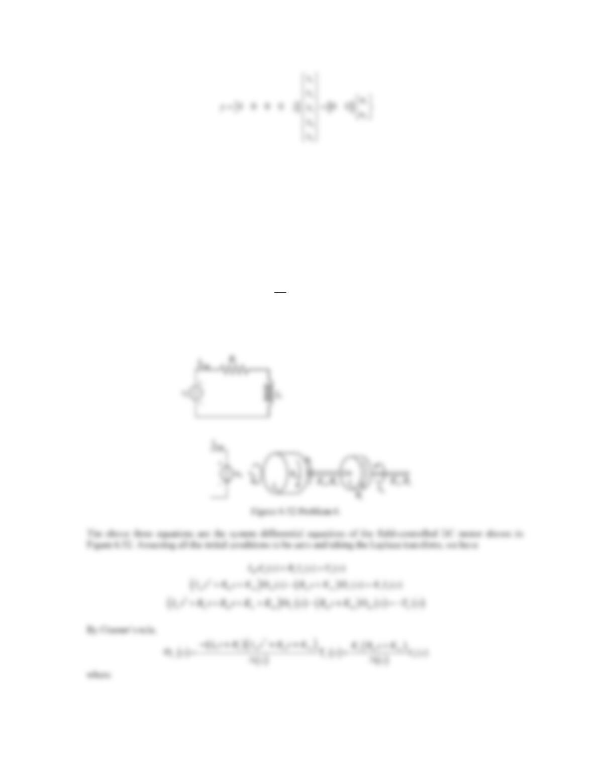
6. A more complicated model of the field-controlled motor is shown in Figure 6.52, where the rotor is connected
to an inertial load through a flexible and damped shaft. Kmand Bmrepresent the torsional stiffness and the
torsional viscous damping of the shaft, respectively. The mass moments of inertia of the motor and the load are
Imand IL, respectively.
a. Derive the transfer functions ȍL(s)/Vf(s)andȍL(s)/TL(s). Assume all of the initial conditions to be zero.
b. Assuming the angular velocity ȦLto be the output, draw a block diagram to represent the dynamics of the
field-controlled motor.
c. Determine the state-space form assuming the angular velocity ȦLto be the output.
Solution
a. Applying Kirchhoff’s current law to the field circuit and the moment equation to the mechanical part gives
f
ffff
di
LRiv
dt
mm m m L m m L m tf
șșș șșIJIB K Ki
LL L m L mm L m L mm L
ș ș ș ș ș IJIBBB KK K
253
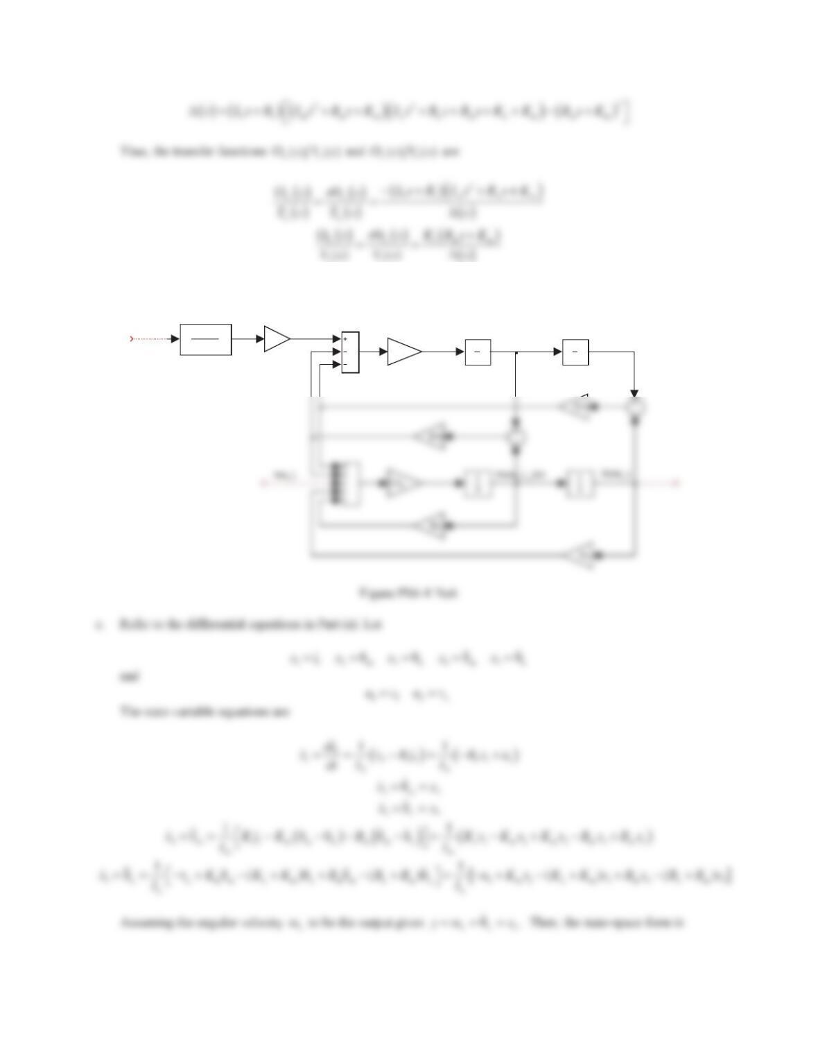
ff
b. A block diagram representing the dynamics of the field-controlled motor is shown below.
theta_m_dot theta_m
i_f tau_m
v_f
1
Lf.s+Rf
1
s
1
s
1/Im
Kt
254
Problem Set 6.5
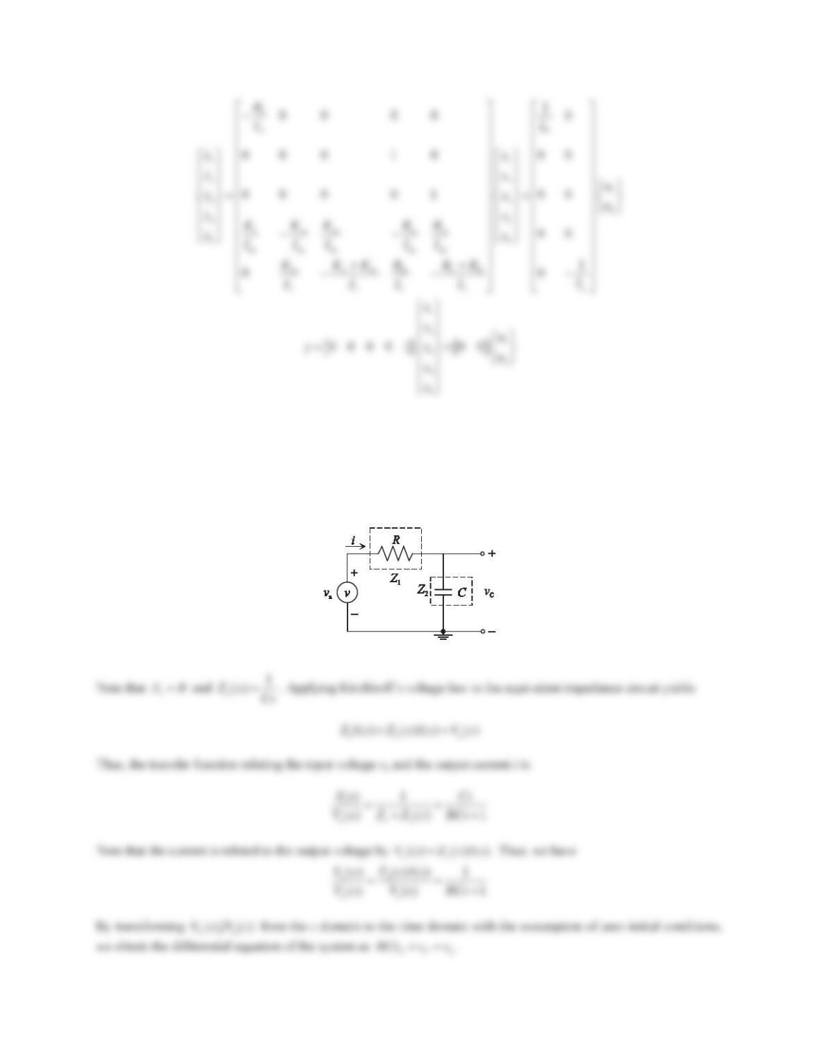
1. Reconsider the RC circuit shown in Figure 6.24. Use the impedance method to determine the transfer function
I(s)/Va(s) and the input–output differential equation relating vCand va. Assume that all the initial conditions are
zero.
Solution
Replacing the passive elements with their impedance representations gives the circuit in the sdomain.
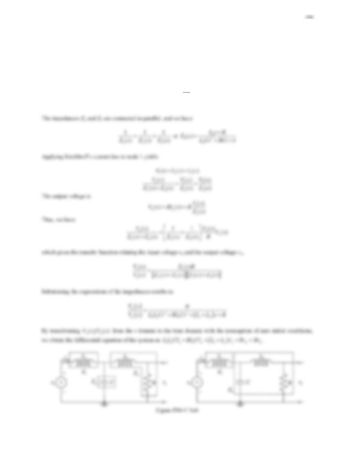
Figure PS6-5 No1
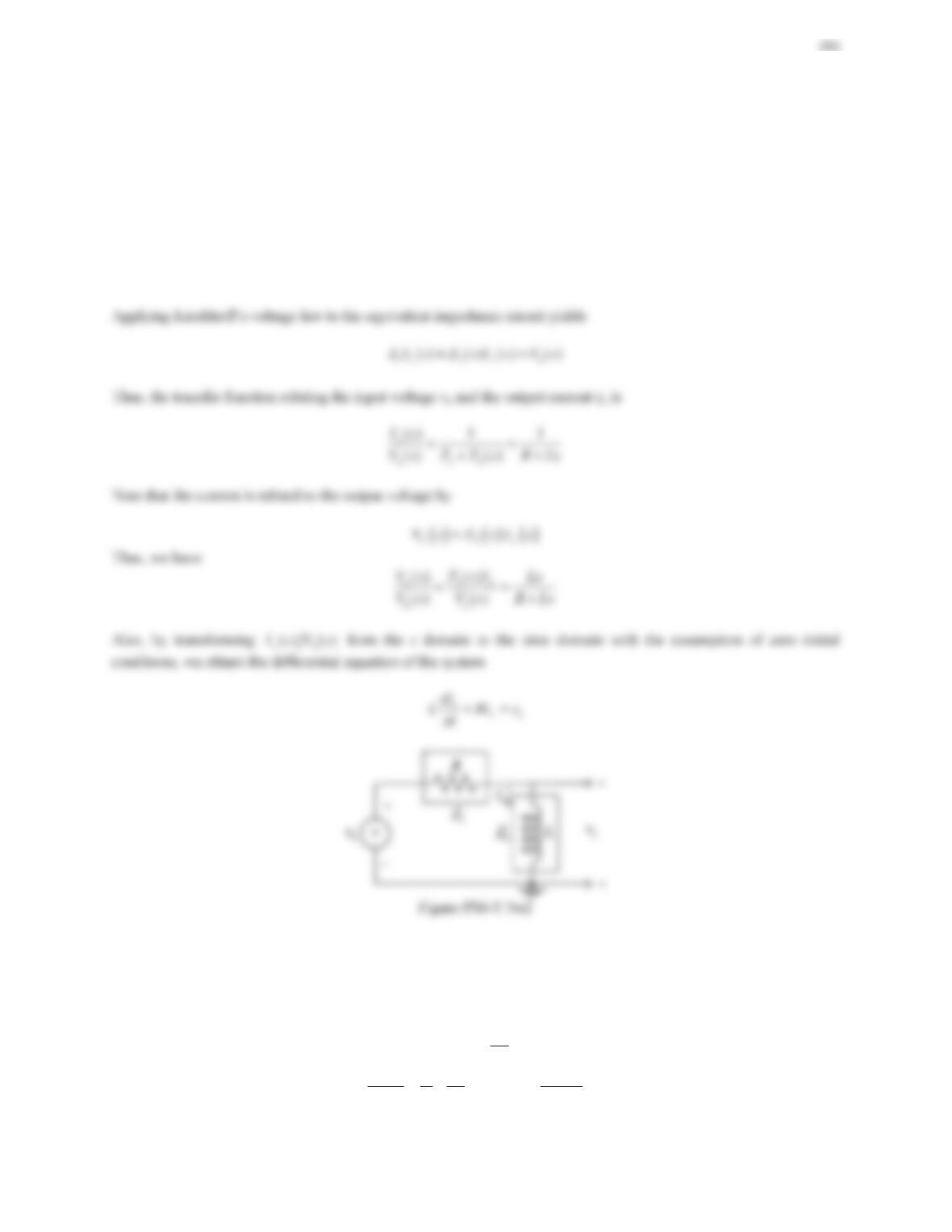
2. Reconsider the RL circuit shown in Figure 6.25. Use the impedance method to determine the transfer function
VL(s)/Va(s) and the input–output differential equation relating iLand va. Assume that all the initial conditions are
zero.
Solution
Replacing the passive elements with their impedance representations gives the circuit in the sdomain as shown in
the figure below, where
1
ZR
2
()Zs Ls
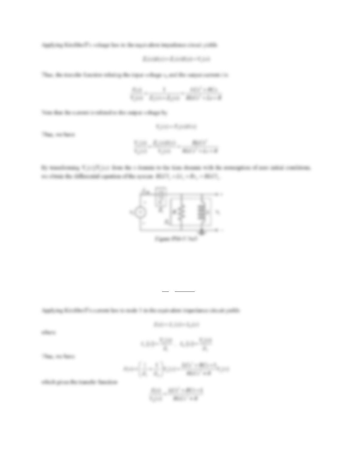
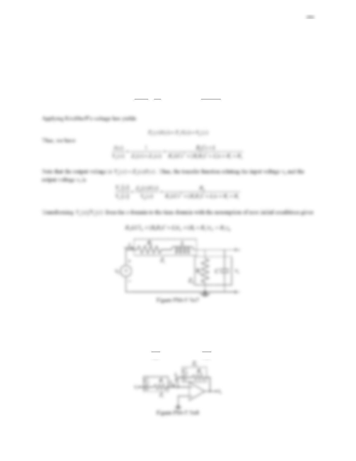
3. Reconsider the RLC circuit shown in Figure 6.26. Use the impedance method to determine the input–output
differential equation relating voand va. Assume that all the initial conditions are zero.
Solution
Replacing the passive elements with their impedance representations gives the circuit in the sdomain as shown in
the figure below, where
1
1
()Zs Cs
2
111
()Zs R Ls
or
2() RLs
Zs Ls R
256
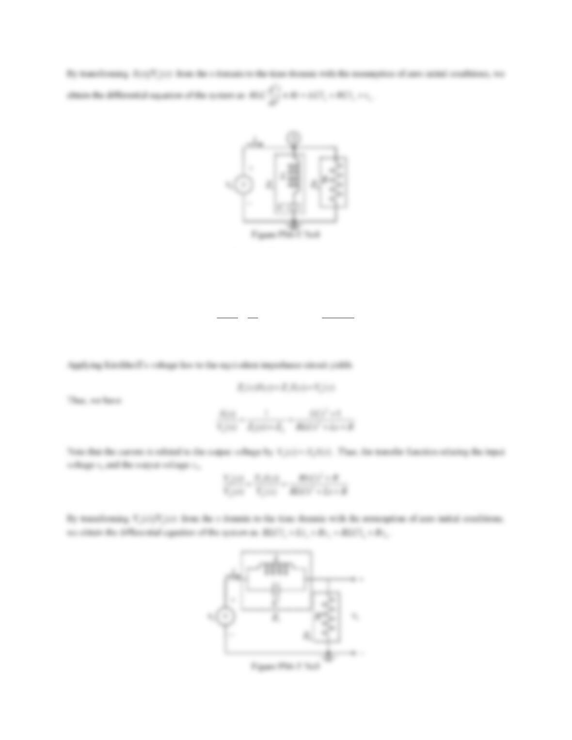
4. Reconsider the RLC circuit shown in Figure 6.27. Use the impedance method to determine the input–output
differential equation relating iand va. Assume that all the initial conditions are zero.
Solution
Replacing the passive elements with their impedance representations gives the circuit in the
s
domain as shown in
the figure below, where
2
1
11
() LCs
Zs Ls Cs Cs
,2
ZR
257
5. Reconsider the RLC circuit shown in Figure 6.28. Use the impedance method to determine the input–output
differential equation relating voand va. Assume that all the initial conditions are zero.
Solution
Replacing the passive elements with their impedance representations gives the circuit in the sdomain as shown in
the figure below, we have
1
11
() Cs
Zs Ls
or
12
() 1
Ls
Zs LCs
2
ZR
6. Reconsider the RLC circuit shown in Figure 6.29. Use the impedance method to determine the input–output
differential equation relating voand va. Assume that all initial conditions are zero.
Solution
Replacing the passive elements with their impedance representations gives the circuit in the sdomain as shown in
the figure below, where
11
()Zs Ls
2
1
()Zs Cs
32
()Zs Ls R
7. Reconsider the RLC circuit shown in Figure 6.30. Use the impedance method to determine the input–output
differential equation relating voand va. Assume that all initial conditions are zero.
Solution
Replacing the passive elements with their impedance representations gives the circuit in the sdomain, where
11
()Zs R Ls
22
11
() Cs
Zs R
or
2
2
2
() 1
R
Zs RCs
8. Reconsider the op-amp circuit shown in Figure 6.41. Use the impedance method to determine the differential
equation relating the input voltage viand the output voltage vo.
Solution
Replacing the passive elements with their impedance representations gives the op-amp circuit in the sdomain as
shown in the figure below, we have
11
1
()Zs R
Cs
and
22
1
()Zs R
Cs
260
Problem Set 6.6
(Note: All MATLAB figures are given at the end of Problem Set 6.6.)
1. Consider the RC circuit shown in Figure 6.24 (Problem Set 6.2, Problem 1), where R = 450 :and C=
1000 PF. When the switch is closed at 1 second, the circuit is driven by a 5V DC voltage source. Assume that
all initial conditions are zero.
a. Build a Simscape model of the physical system and find the loop current i(t) and the voltage across the
capacitor vC(t).
b. Build a Simulink model of the system based on the differential equation relating vCand va, and find the
voltage across the capacitor vC(t).
c. Build a Simulink model of the system based on the transfer function I(s)/Va(s), and find the loop current
i(t).
Solution
The differential equation relating vCand vais
2. Consider the RL circuit shown in Figure 6.25 (Problem Set 6.2, Problem 2), where R = 35 :and L= 10 H.
When the switch is closed at 0 second, the circuit is driven by a 6V DC voltage source. Assume that all initial
conditions are zero.
a. Build a Simscape model of the physical system and find the loop current iL(t) and the voltage across the
inductor vL(t).
b. Build a Simulink model of the system based on the differential equation relating iLand va, and find the loop
current iL(t).
c. Build a Simulink model of the system based on the transfer function VL(s)/Va(s), and find the voltage across
the inductor vL(t).
Solution
The differential equation relating iLand vais
a
()
3. Consider the parallel RLC circuit shown in Example 6.2, where R= 2 :,L= 1 H, and C= 0.5 F. The
circuit is driven by a controlled current source ia(t) = 10u(t), where u(t) is a unit-step function.
a. Build a Simscape model of the physical system and find the voltage across the capacitor vC(t) and the
current through the inductor iL(t).
b. Refer to the results obtained in Example 6.2. Build a Simulink model of the system based on the transfer
function VC(s)/Ia(s) and find the voltage across the capacitor vC(t).
c. Refer to the results obtained in Example 6.2. Build a Simulink model of the system based on the transfer
function IL(s)/Ia(s) and find the current through the inductor iL(t).
Solution
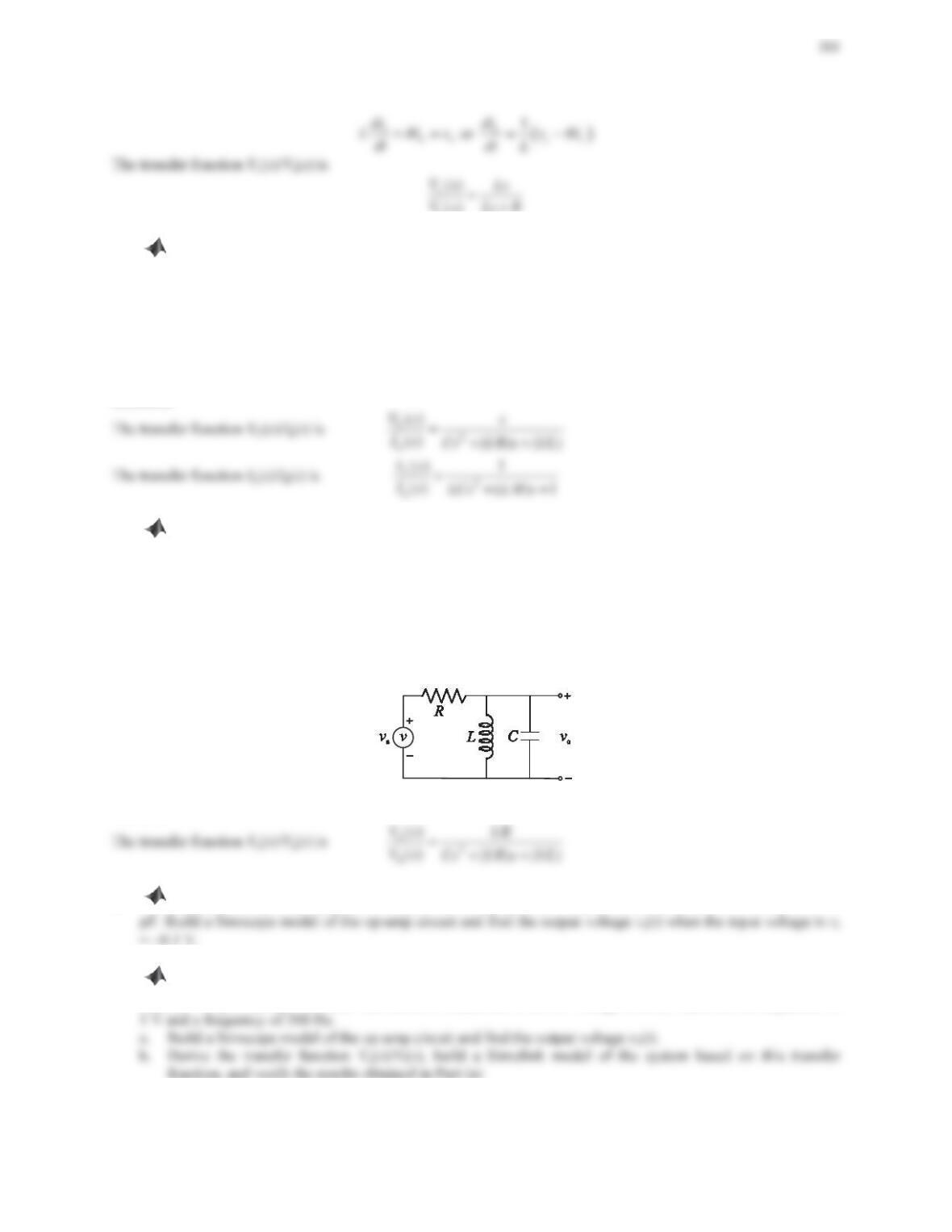
4. A simple band-pass filter can be realized by an RLC circuit (see Figure 6.73), which passes frequencies
within a certain range and attenuates frequencies outside that range. Assume that the parameter values are R=
500 :,L= 100 mH,and C= 10 PF. The circuit is connected to an AC voltage source, which has an amplitude
of 1 V and a varying frequency.
a. Build a Simscape model of the physical system and find the output voltage vo(t) when the frequency of the
input voltage is 1000, 800, and 1200 rad/s.
b. Derive the transfer function Vo(s)/Va(s), build a Simulink model of the system based on this transfer
function, and verify the results obtained in Part (a).
Figure 6.73 Problem 4.
Solution
5. Consider the op-amp integrator in Figure 6.35. Assume that the parameter values are R= 1 M:and C= 1
6. Consider the op-amp circuit shown in Figure 6.74, where the parameter values are C1= 0.8 PF, R1= 10
k:,C2= 80 pF, and R2= 100 k:. The circuit is connected to an AC voltage source, which has an amplitude of