23
In Problems 19–24,
(a) Find the inverse Laplace transform using the partial-fraction expansion method.
(b) Repeat in MATLAB.
19.
34
(1)
s
ss
Solution
(a) Expand as
34
34 ( )
41
(1) 1 (1)
AB A
sABABsA
AB
ss s s ss
20.
2
2
322
(1)(2)
ss
ss
Solution
(a) Partial-fraction expansion leads to
21.
2
10
(25)
s
ss s
Solution
(a) Using partial fractions,
24
22.
22
45
(45)
s
ss s
Solution
(a) Forming partial fractions,
23.
2
8
(2)
s
ss
Solution
(a) Forming partial fractions,
25
24.
2
2
1
(3)( 22)
ss
sss
Solution
(a) Partial-fraction expansion gives
22
22 2
1()(23)23
3
(3)( 22) 22 (3)( 22)
ss A BsC ABs ABCs AC
s
sss ss sss
25.
2 2 ( ) ( 1), (0) 0x x ut ut x
Solution
(a) Taking the Laplace transform and using the zero initial condition, yields
26
26.
1 if 1 2
2 ( ), (0) 0, (0) 0, ( ) 0 otherwise
t
xxxgtxxgt
®
¯
Solution
(a) We first write () ( 1) ( 2)gt ut ut so that
2
()
ss
ee
Gs s
. Laplace transformation of the ODE and using
the zero initial conditions, yields
27
27.
1
3
3 , (0) 0 , (0)
t
xxe x x
Solution
(a) Laplace transformation of the ODE and using the initial conditions leads to
28.
9 sin , (0) 1 , (0) 0xx tx x
Solution
(a) Laplace transform of the ODE and using the initial conditions, we find
29.
2 , (0) 0, (0) 1
t
xx xex x
Solution
(a) Taking the Laplace transform of the ODE and using the given initial conditions, yields
28
30.3 1, (0) 2, (0) 0xx x x
Solution
(a) Taking the Laplace transform of the ODE and using the given initial conditions, yields
2
2
112
( 3 ) ( ) 2 6 ( ) (3)
ssXs s Xs
ss
ss
In Problems 31–36 decide whether the final-value theorem is applicable, and if so, find ss
x.
31.
1
() 2( 3)
Xs ss
Solution
¯¿
32.
2
2
() (4)( 45)
s
Xs sss
Solution
The poles are at
4, 2 j
r
hence the FVT applies.
33.
2
1
() (3)(2)
s
Xs ss s
Solution
34.
2
3
() (2)(1)
s
Xs ss

29
35.
2
2
1
() (1)
s
Xs ss
Solution
The poles are at
0, 1, 1
hence the FVT applies.
36.
1
2
2
() (1)
s
Xs ss s
Solution
The poles are at
3
1
22
0, jr
hence the FVT applies.
In Problems 37–40 evaluate
(0 )x
using the initial-value theorem.
37.
2
2
1
() (2 3)
s
Xs ss s
38.
2
() (1)( 2)
s
Xs ss
39.
(4)
() ( 1)( 2)( 3)
ss
Xs ss s
Solution
40.
2
2
2
() (3 1)( 9)
s
Xs ss
30
Review Problems
In Problems 1–4 perform the operations and express the result in rectangular form.
1.
2
(1 3 )
2
j
j
Solution
2.
1
3
1
2(3 2)
j
jj
3.
5
(0.6 0.8 )j
Solution
Since
0.9273
0.6 0.8 j
je
, we have
4.
4
3
(1 3 )
(3 )
j
j
Solution
5. Find all possible values of
1/3
3
2
3j
.
Solution
Let
2.6779
35
3
22
3j
zje
so that
35
2
r
and
2.6779 rad
T
. With 3n , Eq. (2.9) yields
6. Find all possible values of
1 0.3j
.
Solution
Let
0.2915
1 0.3 1.0440
j
zj e
so that 1.0440r and
0.2915 rad
T
. With 2n , Eq. (2.9) gives
r
7. Solve the initial-value problem 3 2 , (0) 4yy ty
.
Solution
Rewrite in standard form as 12
33
yyt
so that by Eq. (2.12),
8.Express
cos 2sintt
in the form cos( )Dt
I
for suitable amplitude
D
and phase
I
.
Solution
Expand
cos( ) cos cos sin sinDt Dt Dt
III
. Comparing with
cos 2sintt
, we find
9. Solve the initial-value problem
3
3 3 , (0) 0, (0) 2
t
xxe x x
using
(a) the method of undetermined coefficients,
(b) Laplace transformation.
Solution
(a) The characteristic equation
230
OO
yields .. so that
3
()
t
h
xt ABe
. Because the function on the right
side of the ODE matches a homogeneous solution, pick
3t
p
xkte
and insert into the ODE to find
33K
, hence
10. Solve the initial-value problem
2 ( 1), (0) 0, (0) 1xx t x x
G
.
Solution
Taking the Laplace transform of the ODE and using the initial conditions, we find
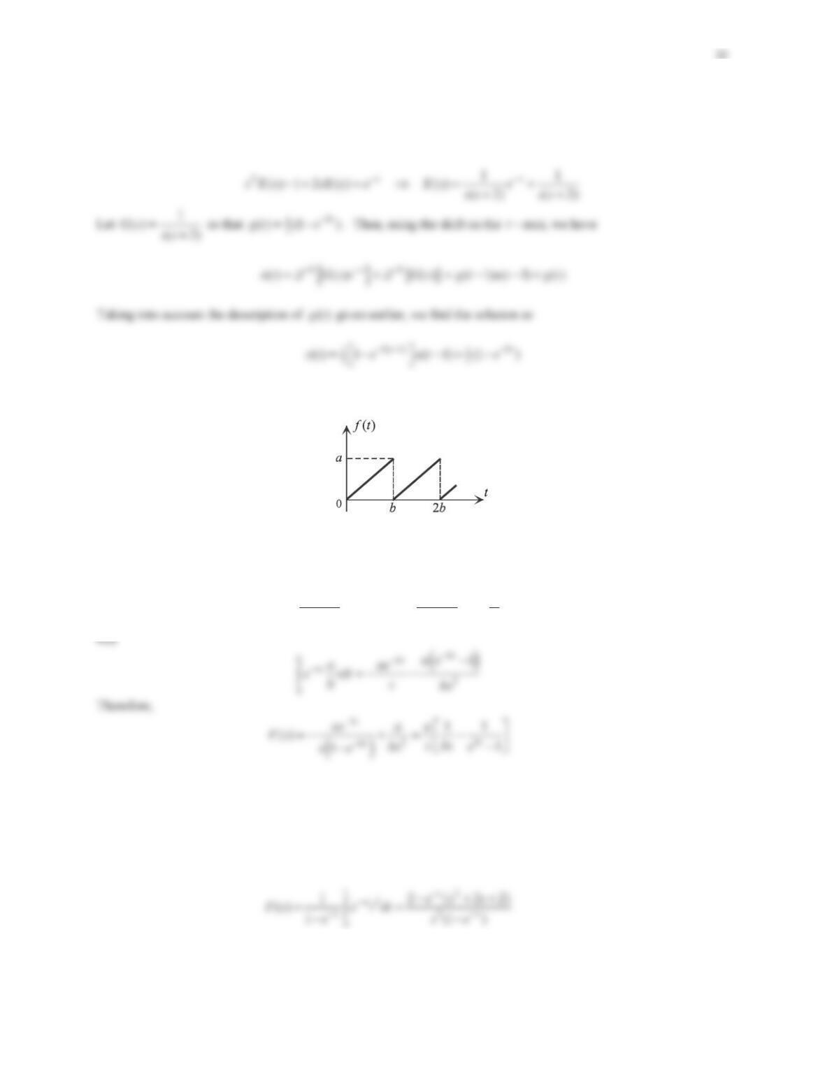
11. Find the Laplace transform of the periodic function in Figure 2.16.
Figure 2.16 Problem 11.
Solution
The period is
Pb
. Using the description of ()ft, we have
00
11
() ()
11
bb
st st
bs bs
a
Fs e ftdt e tdt
b
ee
³³
12. Find the Laplace transform of the periodic function whose definition in one period is
2
() , 0 1ft t t
Solution
The period is
1P
. Using the description of ()ft, we have
13. Evaluate the convolution
()ut a t
.
33
a
14. Find the convolution
(1) t
ut e
.
15. Using partial-fraction expansion, find
2
1
22
21
(4 1)
s
ss
½
°°
®¾
°°
¯¿
L
Solution
Partial-fraction expansion results in
16. Using convolution, find
1
2
2
(1)( 1)
s
ss
½
°°
®¾
°°
¯¿
L
Solution
Writing the transform function as the product of
2
1s
and
21
s
s
, and noting that their inverse Laplace transforms
are
2t
e
and
cos t
, we have
17. Consider
2
1
() (1)
Xs ss
(a) Using the final-value theorem, if applicable, evaluate
ss
x
.
(b) Confirm the result of Part (a) by evaluating
^`
lim ( )
t
xt
of
.
34
Solution
(a) Poles of ()Xs are at
0, 1, 1
so that the FVT is applicable:
18. Repeat Problem 17 for
2
0.1
() ( 0.2 25.01)
s
Xs ss s
.
Solution
(a) Poles of ()Xs are at
0, 0.1 5 jr
so that the FVT is applicable:
19. Consider
2
3
() 2( 0.4 1.04)
s
Xs ss
(a) Using the initial-value theorem, evaluate
(0 )x
.
(b) Confirm the result of Part (a) by evaluating
^`
0
lim ( )
t
xt
o
.
Solution
(a)
^`
2
2
33
(0 ) lim ( ) lim 2
2( 0.4 1.04)
ss
s
xsXs
ss
of of
20.Assuming
2
0.4 0.3
() (3 1)
s
Xs ss
, evaluate
(0 )x
using the initial-value theorem.
Solution