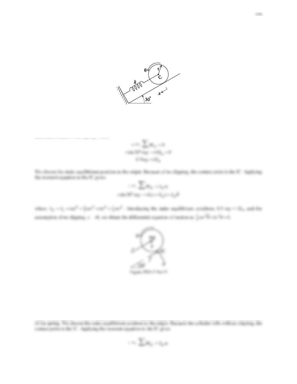
15. Consider the system shown in Figure 5.73, where a uniform sphere of mass mand radius rrolls along an
inclined plane of 30°. A translational spring of stiffness kis attached to the sphere. Assuming that there is no
slipping between the sphere and the surface, draw the necessary free-body diagram and derive the differential
equation of motion.
Figure 5.73 Problem 15.
Solution
The free-body diagram of the system is shown in the figure below, where the normal force Nand the friction force f
are reaction forces at the contact point. Assuming that the sphere rolls down the incline, the spring is in compression
and fkis the spring force. When the sphere is at the static equilibrium position, we have fk=kįst ZKHUHįst is the
static deformation of the spring. Then,
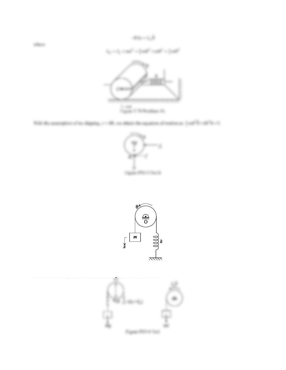
16. Consider the system shown in Figure 5.74. A uniform solid cylinder of mass m, radius R, and length Lis fitted
with a frictionless axle along the cylinder’s long axis. A spring of stiffness kis attached to a bracket connected
to the axle. Assume that the cylinder rolls without slipping on a horizontal surface. Draw the necessary free-
body diagram and derive the differential equation of motion.
Solution
The free-body diagram of the system is shown, where the normal force Nand the friction force fare reaction forces
at the contact point. When the cylinder is at the static equilibrium position, Gst = 0, where Gst is the static deformation
175
Problem Set 5.4
1. For the pulley system in Example 5.14, draw the free-body diagram and kinematic diagram, and derive the
equation of motion using the force/moment approach.
Figure 5.82 A pulley system.
Solution
The free-body diagram and the kinematic diagram are shown below.
176
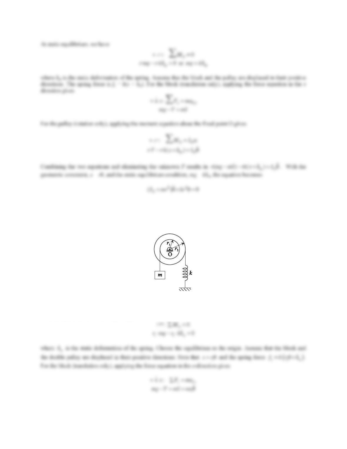
2. The double pulley system shown in Figure 5.86 has an inner radius of r1and an outer radius of r2. The mass
moment of inertia of the pulley about point O is IO. A translational spring of stiffness kand a block of mass m
are suspended by cables wrapped around the pulley as shown. Draw the free-body diagram and kinematic
diagram, and derive the equation of motion using the force/moment approach.
Figure 5.86 Problem 2.
Solution
The free-body diagram and the kinematic diagram are shown below.
At static equilibrium, we have
st
į
k
fk
and
177
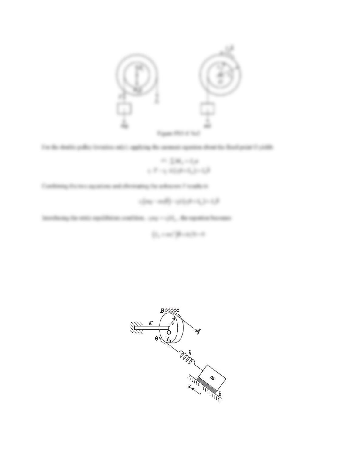
3. Consider the mechanical system shown in Figure 5.87. A disk-shaft system is connected to a block of mass m
through a translational spring of stiffness k. The elasticity of the shaft and the fluid coupling are modeled as a
torsional spring of stiffness Kand a torsional viscous damper of damping coefficient B, respectively. The radius
of the disk is rand its mass moment of inertia about point O is IO. Assume that the friction between the block
and the horizontal surface cannot be ignored and is modeled as a translational viscous damper of damping
coefficient b. The input to the system is the force f. Draw the necessary free-body diagram and the kinematic
diagram, and derive the equations of motion.
Figure 5.87 Problem 3.
178
Solution
This is a mixed system, where the mass block undergoes translational motion along x-direction and the motion of the
disk is pure rotation about point O that is fixed. Choose the displacement of the block xand the angular
displacement of the disk șDVWKHJHQHUDOL]HGFRRUGLQDWHVAssuming that the block and the disk are displaced in their
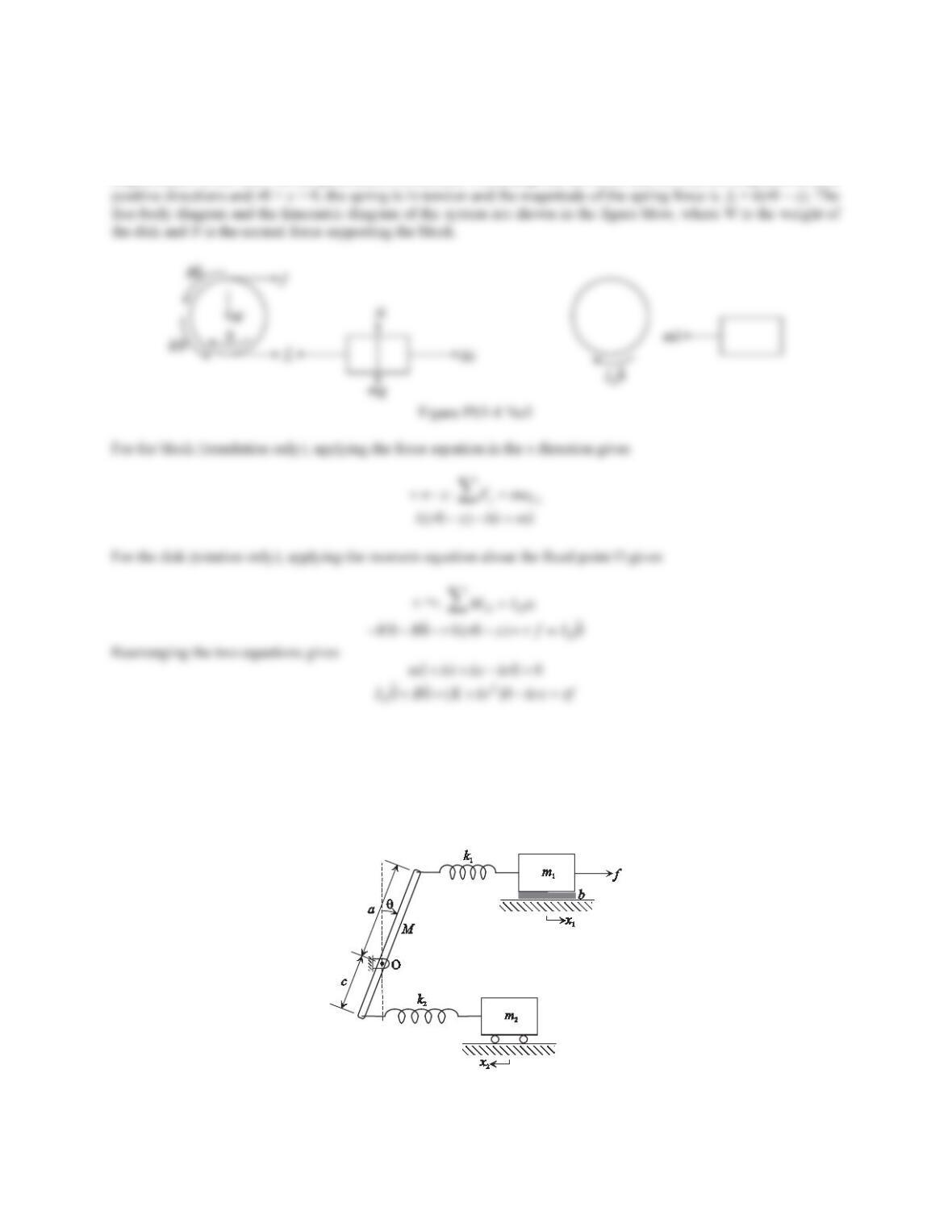
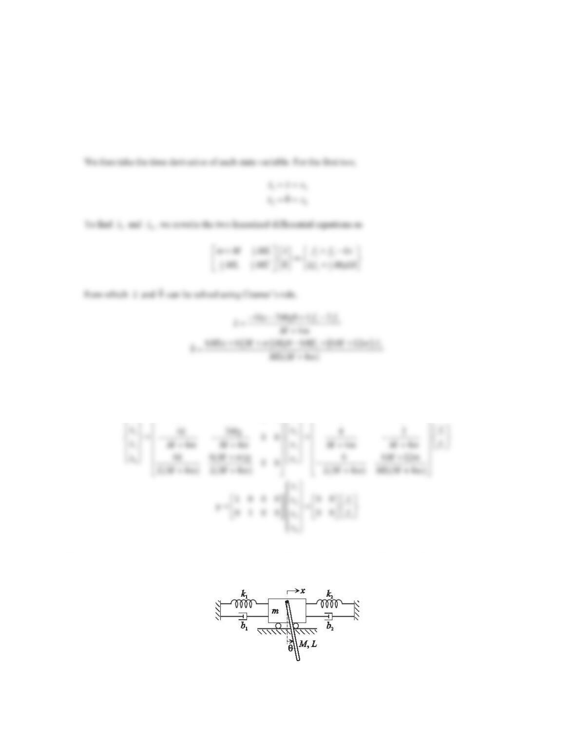
4. Consider the mechanical system shown in Figure 5.88, where the motion of the rod is small angular rotation.
When T= 0 and f= 0, the deformation of each spring is zero and the system is at static equilibrium. Assume that
the friction between the block of mass m1and the horizontal surface cannot be ignored and is modeled as a
translational viscous damper of damping coefficient b.
a. Assuming that a>c> 0, determine the mass moment of inertia of the rod about the pivot point O.
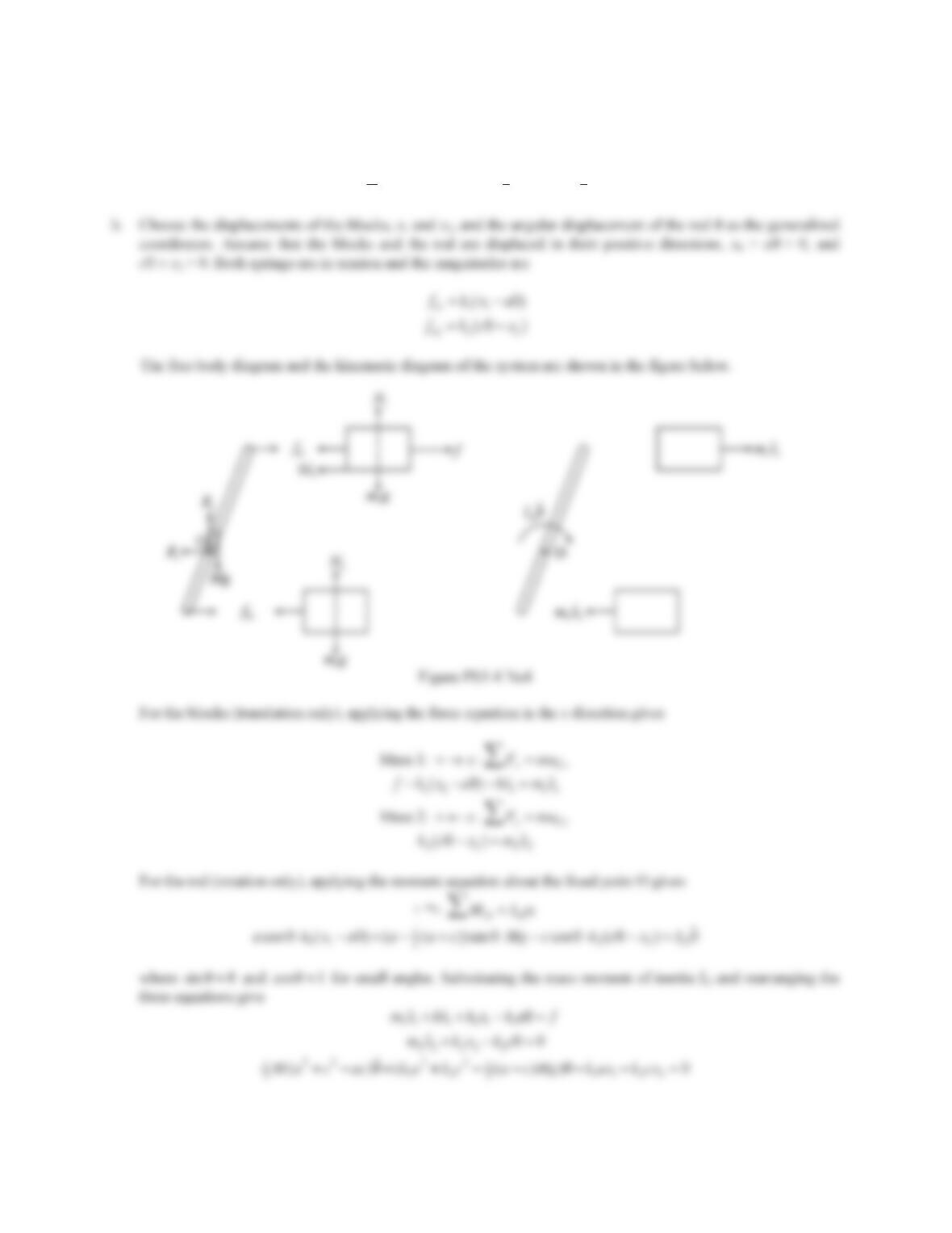
b. Draw the necessary free-body diagram and the kinematic diagram, and derive the equations of motion for
small angles.
Figure 5.88 Problem 4.
179
Solution
a. The mass moment of inertia of the rod about point O can be found by applying the parallel axis theorem
2
22 22
111
OC 12 2 3
() () ( )IIMd MacMa ac Macac
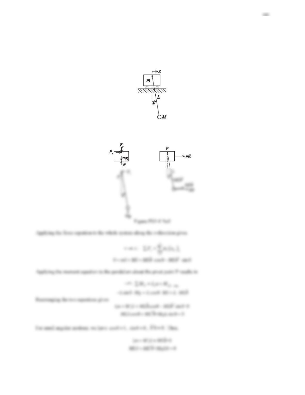
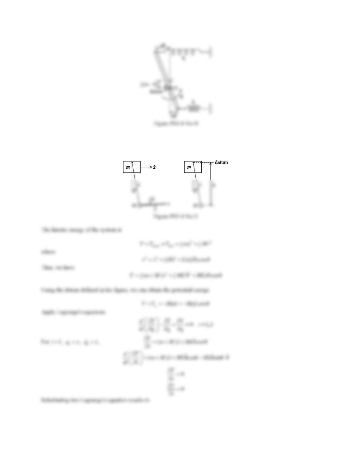
5. Consider the mechanical system shown in Figure 5.89, where a simple pendulum is pivoted on a cart of mass m.
The pendulum consists of a point mass Mconcentrated at the tip of a massless rod of length L. Assume that the
pendulum is constrained to rotate in a vertical plane, and the cart moves on a smooth horizontal surface. Denote
the displacement of the cart as xDQGWKHDQJXODUGLVSODFHPHQWRIWKHSHQGXOXPDVș‘UDZWKHQHFHVVDU\IUHH–
body diagram and kinematic diagram, and derive the equations of motion for small angles.
Figure 5.89 Problem 5.
Solution
The free-body diagram and the kinematic diagram are shown in the figure below.
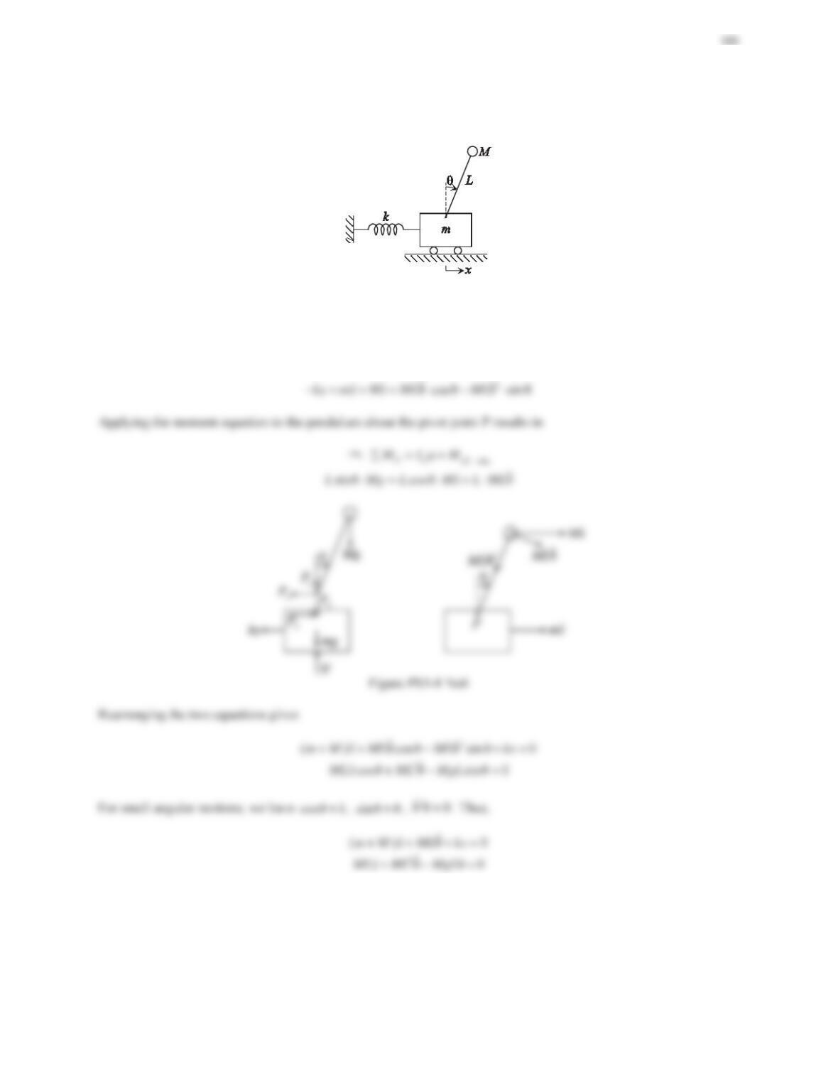
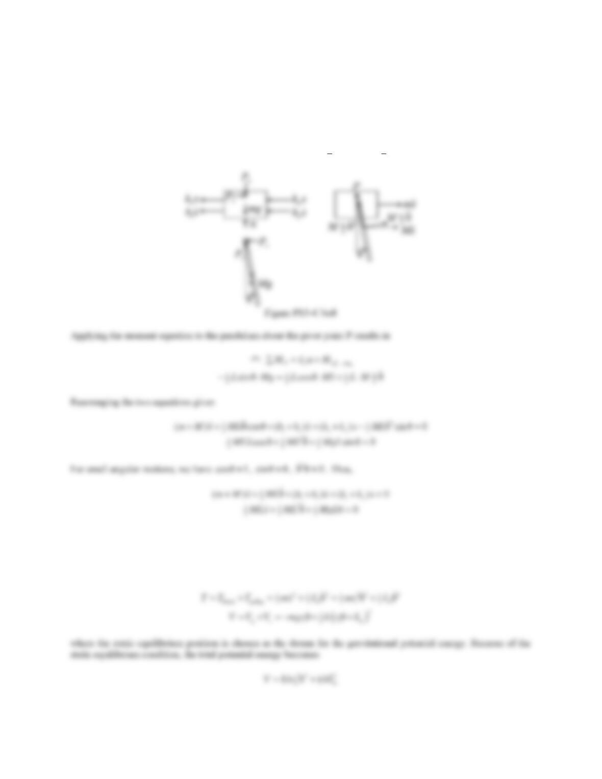
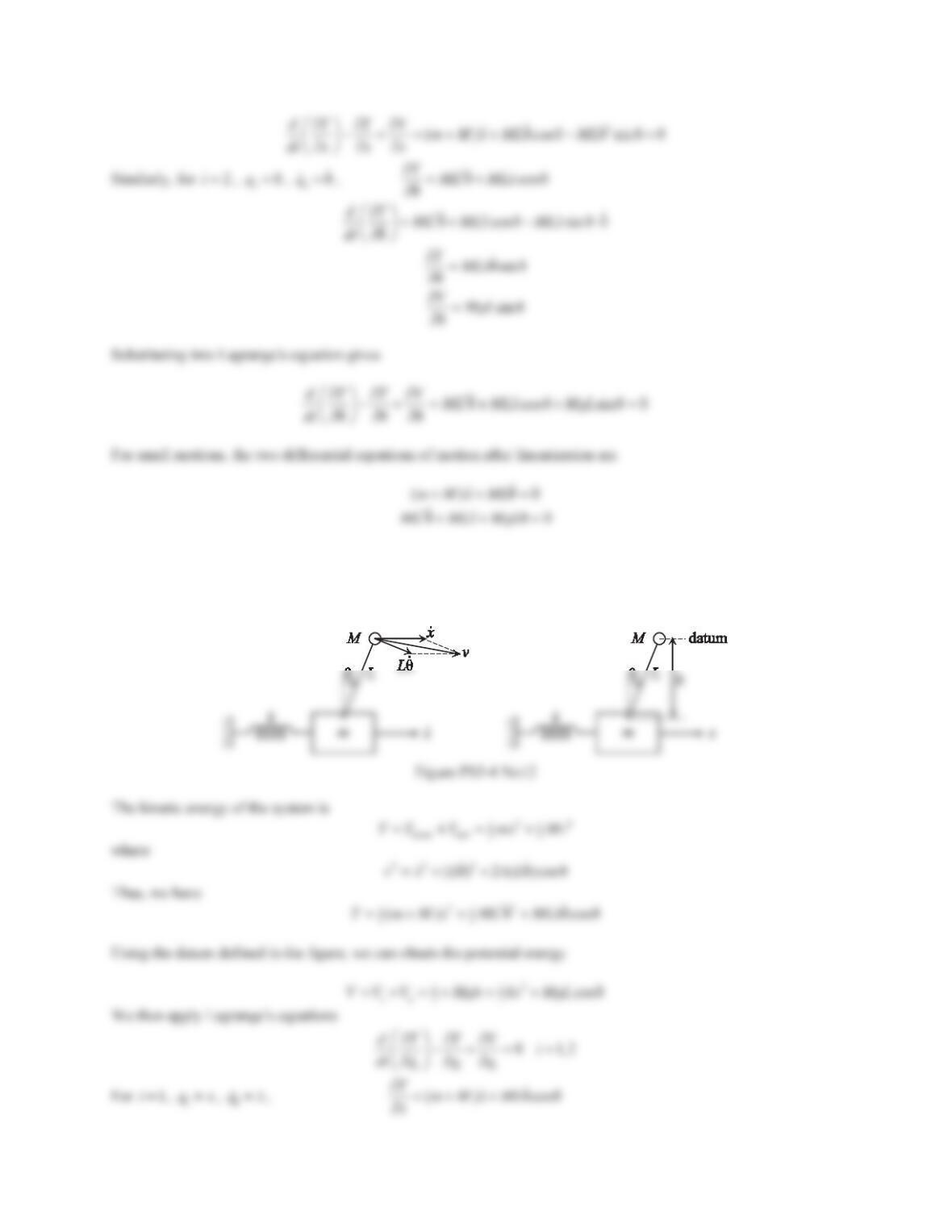
6. Consider the mechanical system shown in Figure 5.90. Draw the necessary free-body diagram and kinematic
diagram, and derive the equations of motion for small angles.
Figure 5.90 Problem 6.
Solution
The free-body diagram and the kinematic diagram are shown in the figure below. Applying the force equation to the
whole system along the x-direction gives
2
1
:
xiCi
x
i
xF ma
o ¦ ¦
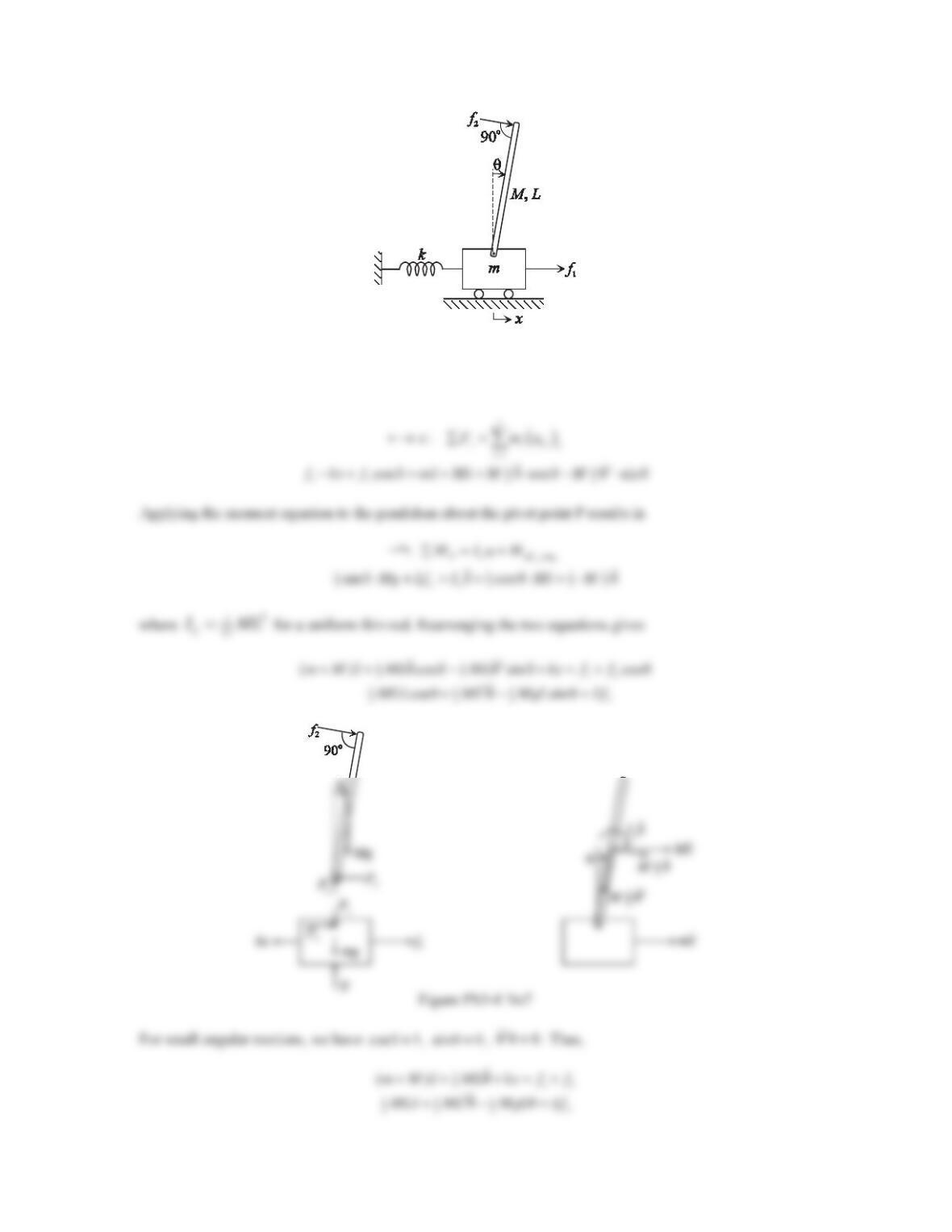
7. Consider the mechanical system shown in Figure 5.91. The inputs are the force f1applied to the cart and the
force f2applied at the tip of the rod. The outputs are the displacement xof the cart and the angular displacement
șRIWKHSHQGXOXP
a. Draw the free-body diagram and kinematic diagram, and derive the equations of motion for small angles.
b. Using the differential equation obtained in Part (a), determine the state-space representation.
182
Figure 5.91 Problem 7.
Solution
a. The free-body diagram and the kinematic diagram are shown in the figure below.
Applying the force equation to the whole system along the x-direction gives
183
b. The state, the input, and the output are specified as
1
21
32
4
ș
ș
ș
xx
xf
x
xf
x
x
½½
°°°° ½ ½
°°°°
® ¾ ®¾ ® ¾ ®¾
¯¿
¯¿
°°°°
°°°°
¯¿
¯¿
xuy
Thus, the state-space equation in matrix form is
11
0010 0 0
0001 0 0
xx
ªºªº
«»«»
½ ½
8. Consider the mechanical system shown in Figure 5.92. Draw the necessary free-body diagram and kinematic
diagram, and derive the equations of motion for small angles.
Figure 5.92 Problem 8.
184
Solution
The free-body diagram and the kinematic diagram are shown in the figure below. Applying the force equation to the
whole system along the x-direction gives
2
1
:
xiCi
x
i
xF ma
o ¦ ¦
2
11 2 2 22
șFRVș ș VLQș
LL
kx bx kx bx mx Mx M M
9. For the mechanical system in Problem 2, use the energy method to derive the equation of motion.
Solution
The static equilibrium position and the deformed positions are shown in the figure below. At equilibrium, we have
12st
įrmg rk
. Assuming that the block and the pulley move along the direction shown gives
185
10. For the mechanical system in Problem 11 of Problem Set 5.3, use the energy method to derive the equation of
motion.
Solution
The system is only subjected to the gravitational and spring forces, and it is a conservative system. When ș , the
springs are at their free length. Assuming that the rod rotates along the positive direction by a small angle Tgives
2
1
O
2
șTI
22
111
12
222
()cosșș ș
ge
VV V Mg ab ka kb
186
11. Repeat Problem 5 using Lagrange’s equations.
Solution
The system is only subjected to the gravitational forces, and it is a conservative system.
187
12. Repeat Problem 6 using Lagrange’s equations.
Solution
The system is only subjected to the gravitational and spring forces, and it is a conservative system.
188
13. A robot arm consists of rigid links connected by joints allowing the relative motion of neighboring links. The
dynamic model for a robot arm can be derived using Lagrange’s equations
d,1,2,,
d
i
ii
i
TTV
in
t
§·
www
W }
¨¸
¨¸
wT wT
wT
©¹
ZKHUHșiis the angular displacement of the iWKMRLQWIJiis the torque applied to the ith joint, and nis the total
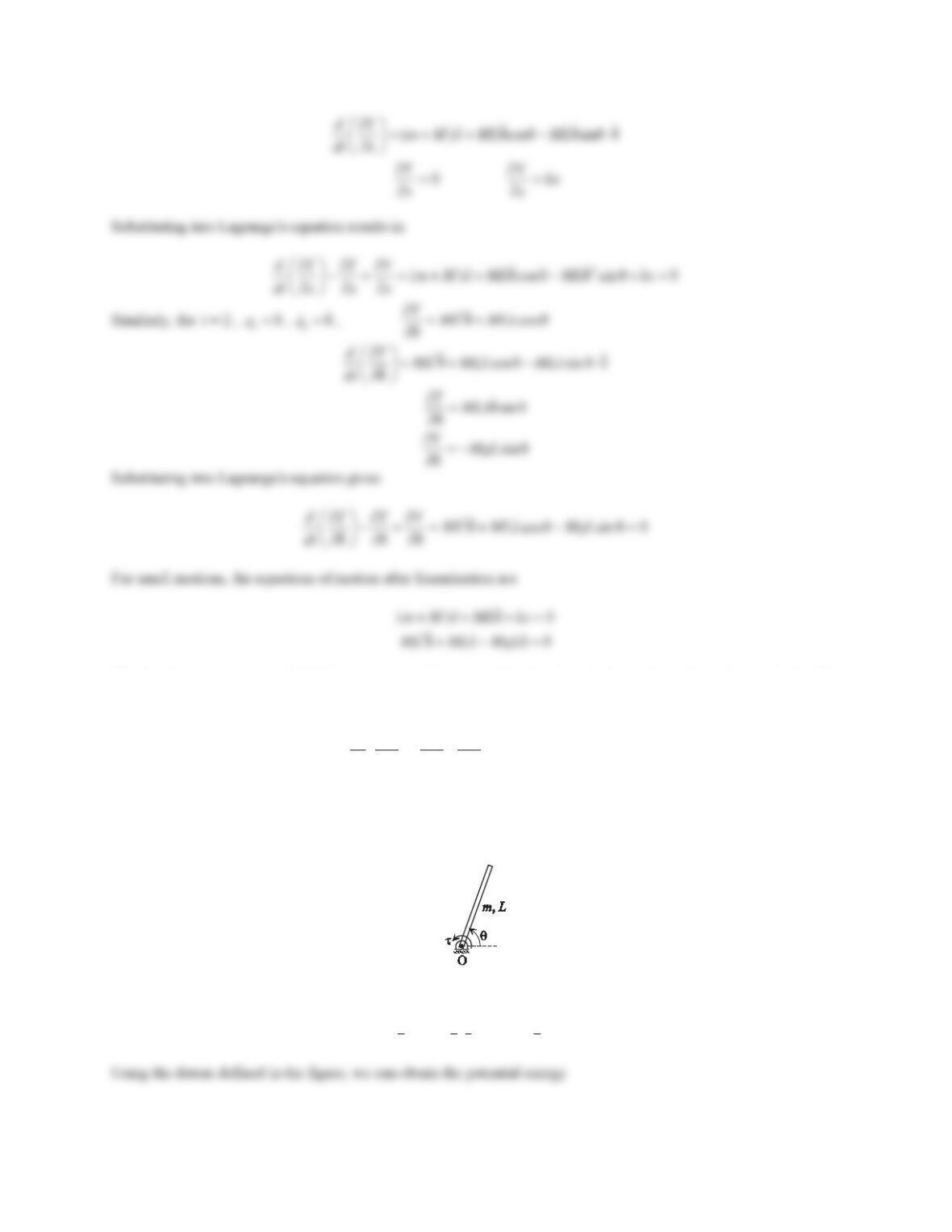
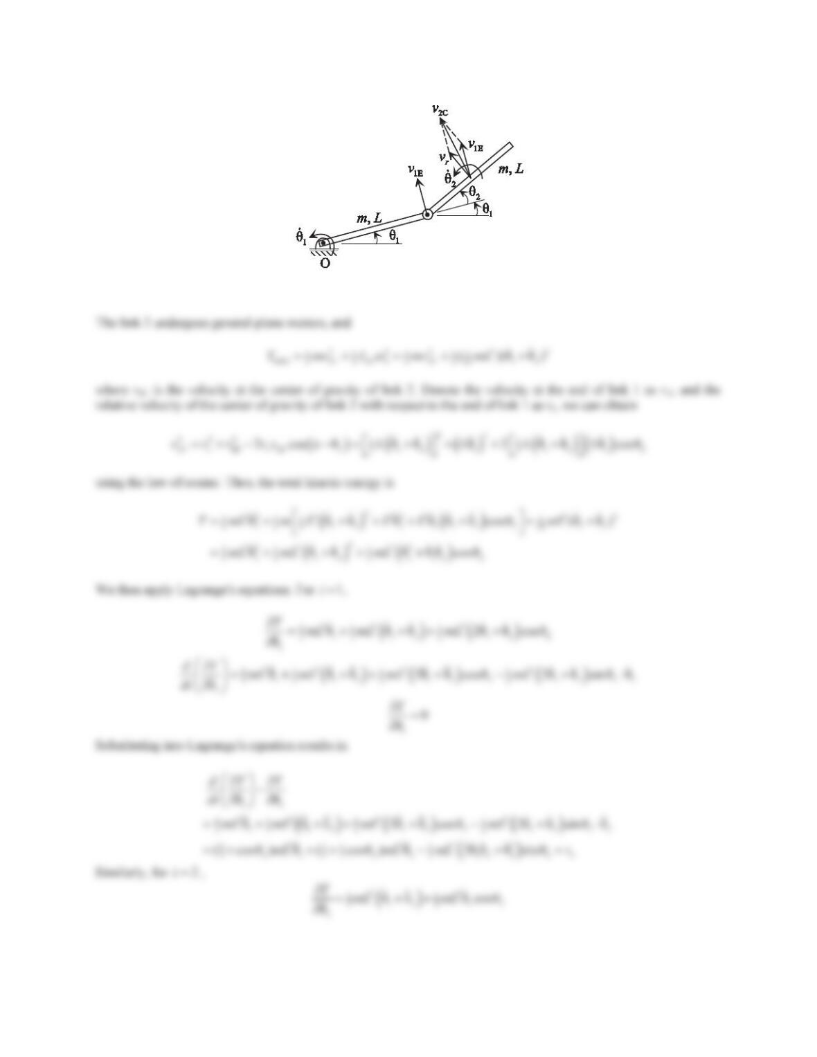
number of joints. Consider a single-link planar robot arm as shown in Figure 5.93. Use Lagrange’s equations to
derive the dynamic model of the robot arm. Assume that the motion of the robot arm is constrained in a vertical
plane, and the joint angle varies between 0° and 360°.
Figure 5.93 Problem 13.
Solution
The kinetic energy of the robot arm is
22222
111 1
O
223 6
ș ș șT I mL mL
189
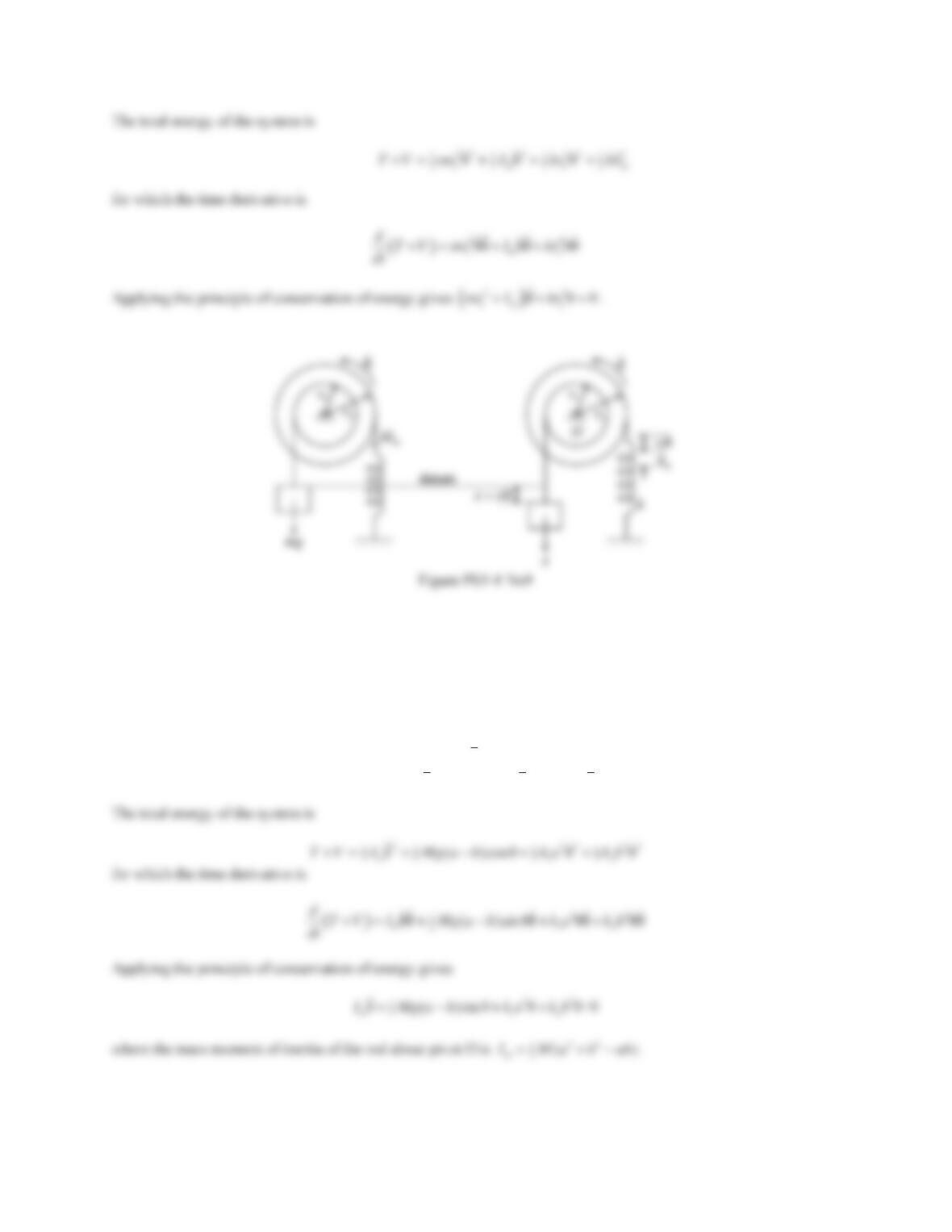
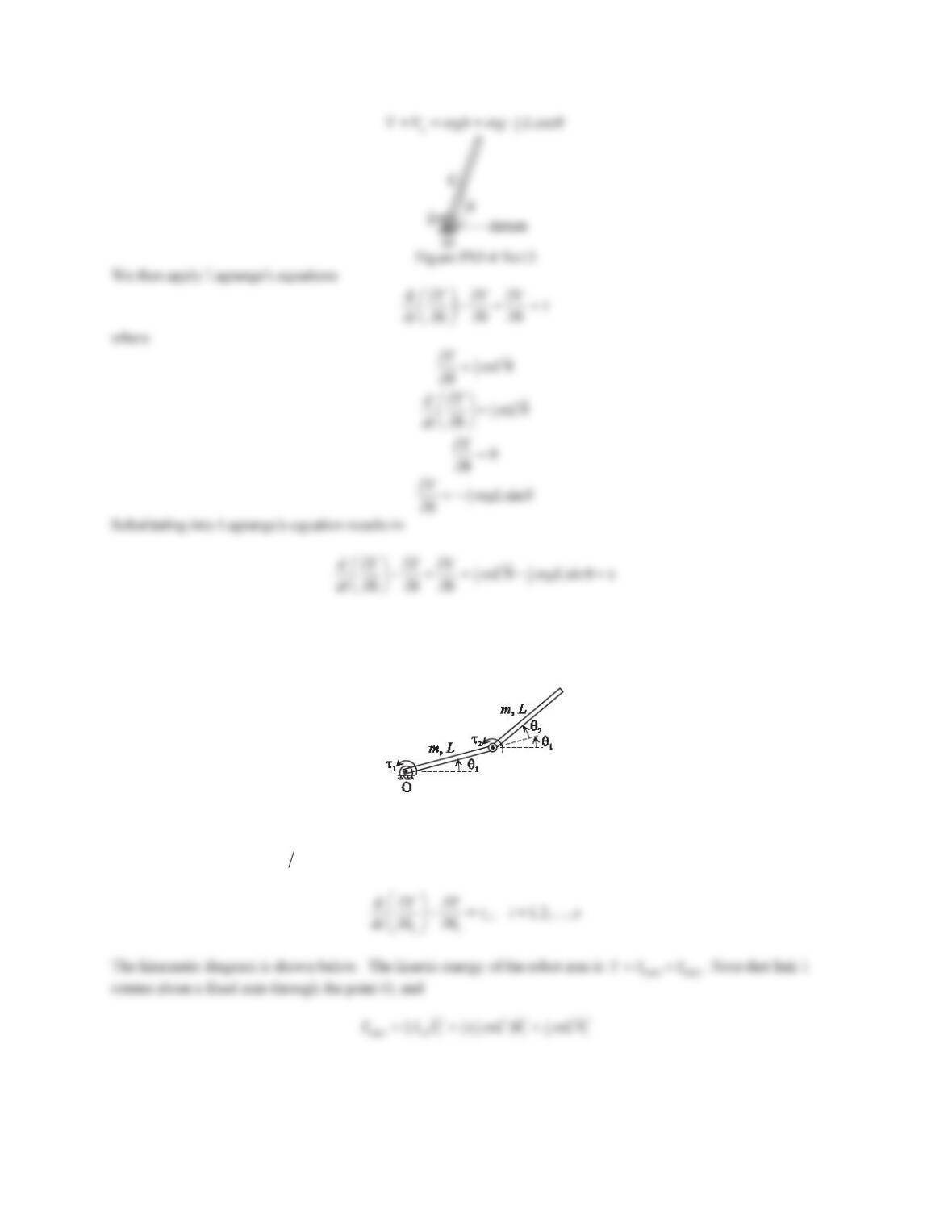
14. Repeat Problem 13 for a two-link planar robot arm as shown in Figure 5.94. Assume that the motion of the
robot arm is constrained in a horizontal plane, and the joint angles vary between 0° and 360°.
Figure 5.94 Problem 14.
Solution
The motion of the robot arm is assumed to be constrained in a horizontal plane. Thus, the gravitational potential
energy does not change ( ș
i
Vww
) and the Lagrange’s equations can be rewritten as
190
Figure PS5-4 No14
191
Problem Set 5.5
1. Repeat Example 5.16, and determine a mathematical model for the simple one-degree-of-freedom system
shown in Figure 5.95DLQWKHIRUPRIDGLIIHUHQWLDOHTXDWLRQRIPRWLRQLQș2.
Solution
As shown in Example 5.16, the differential equation of motion in
1
ș
is
2
1
C1 C2 1 1
2
2
r
II
r
§·
T W
¨¸
¨¸
©¹
Introducing the geometric constraint
21 12
rrTT
,the above differential equation can be rewritten as
2. Repeat Example 5.17, and determine a mathematical model for the single-link robot arm shown in Figure 5.96
LQWKHIRUPRIDGLIIHUHQWLDOHTXDWLRQRIPRWLRQLQWKHORDGYDULDEOHș
192
Solution
As shown in Example 5.17, the differential equation of motion in terms of the angular displacement of the motor is
22
mmm mm
()( )INI BNBT T W
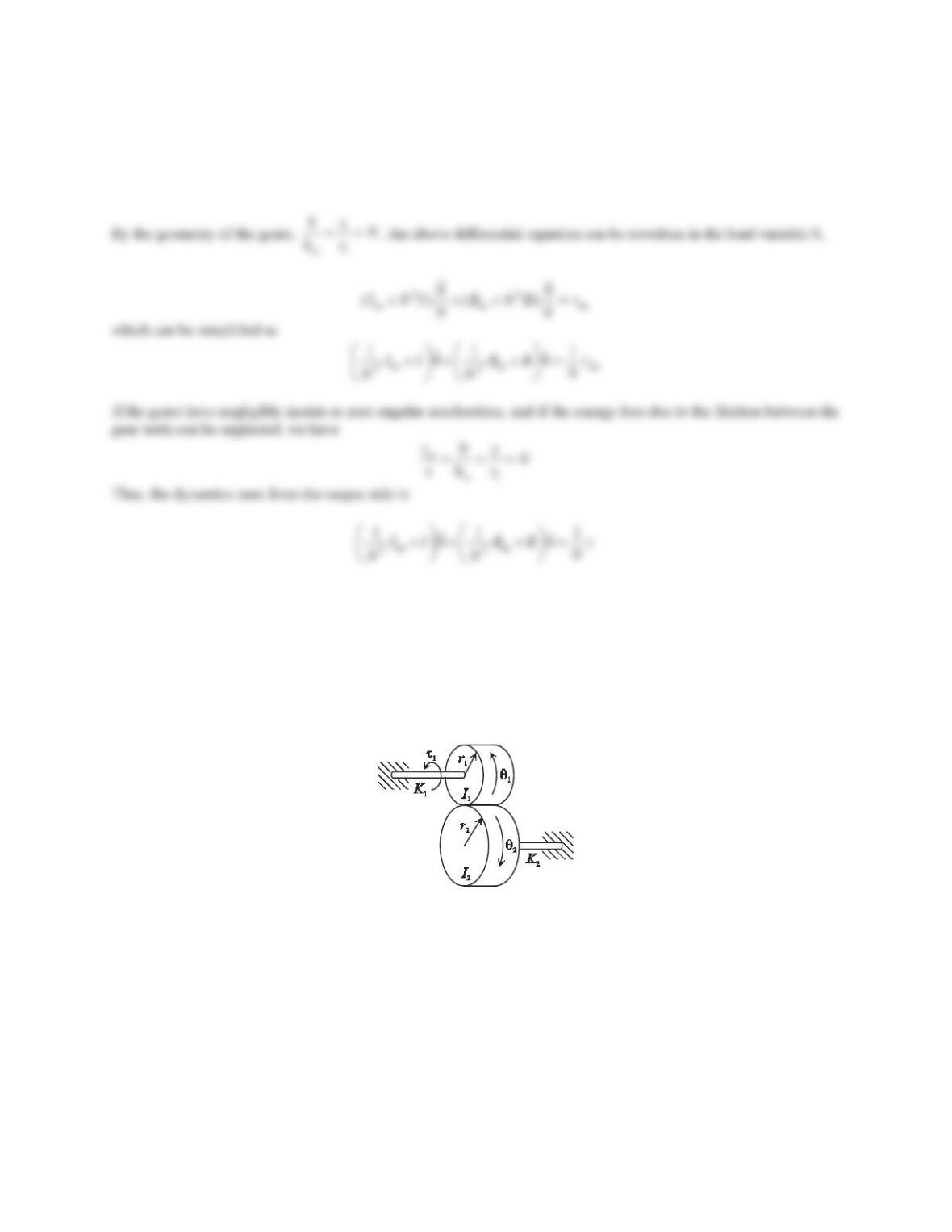
3. Consider the one-degree-of-freedom system shown in Figure 5.98. The system consists of two gears of mass
moments of inertia I1and I2and radii r1and r2UHVSHFWLYHO\7KHDSSOLHGWRUTXHRQJHDULVIJ1. Assume that the
gears are connected with flexible shafts, which can be approximated as two torsional springs of stiffnesses K1
and K2, respectively.
a. Draw the necessary free-ERG\GLDJUDPVDQGGHULYHWKHGLIIHUHQWLDOHTXDWLRQRIPRWLRQLQș1.
b. 8VLQJWKHGLIIHUHQWLDOHTXDWLRQREWDLQHGLQ3DUWDGHWHUPLQHWKHWUDQVIHUIXQFWLRQĬ2(s)/T1(s).
c. Using the differential equation obtained in Part (a), determine the state–VSDFHUHSUHVHQWDWLRQZLWKș2as the
output.
Figure 5.98 Problem 3.
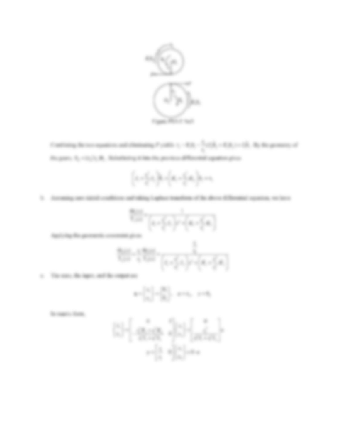
Solution
a. The free-body diagram is shown in the figure below. Applying the moment equation to each gear gives
+:
OO
ĮMI¦
Gear 1:
1111 11
IJș șKrFI
Gear 2:
22 2 22
șșKrFI
193
4. Consider the gear–train system shown in Figure 5.99. The system consists of a rotational cylinder and a pair of
gears. The gear ratio is N=r1/r27KHDSSOLHGWRUTXHRQWKHF\OLQGHULVIJa. Assume that the gears are connected
with flexible shafts, which can be approximated as two torsional springs of stiffnesses K1and K2, respectively.
a. Draw the necessary free-body diagrams, and derive the differential equations of motion.