Unlock document.
This document is partially blurred.
Unlock all pages and 1 million more documents.
Get Access
311
Problem Set 8.1
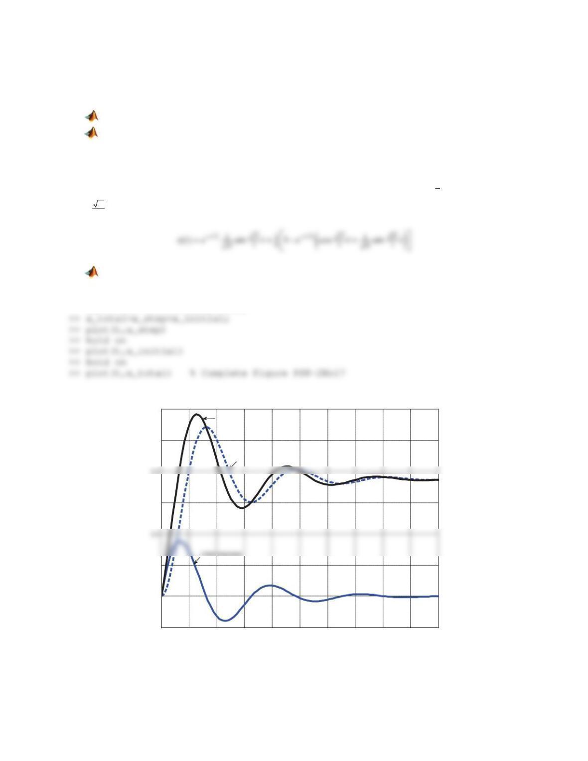
1. Consider a first-order system with time constant
W
and zero initial condition. Find the system’s unit-impulse
response for
1
4
W
and
1
2
W
, plot the two curves versus
02tdd
in the same graph, and comment.
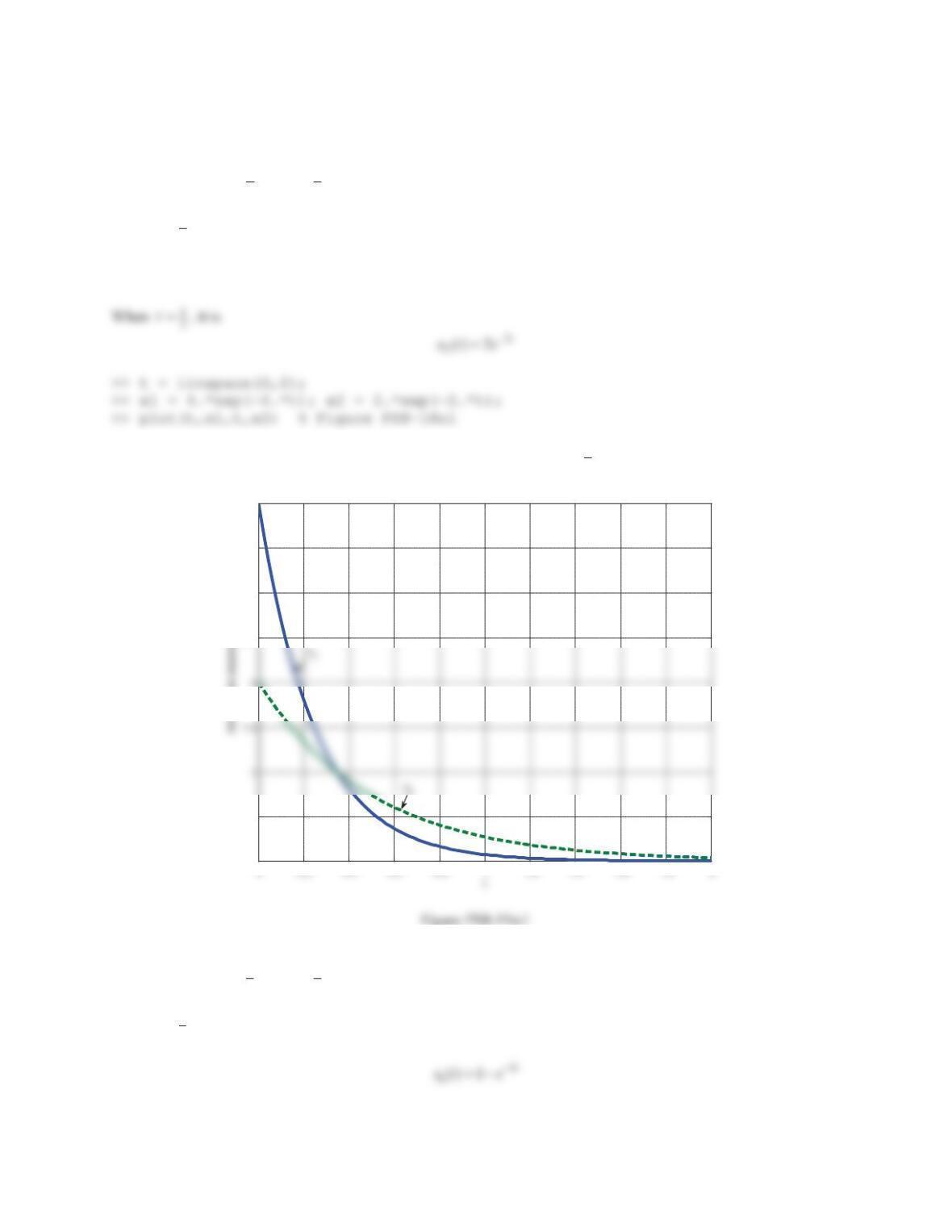
Solution
When
1
4
W
, the unit-impulse response is
4
1() 4 t
xt e
As expected, the response
1
x
associated with the smaller time constant
1
4
W
reaches steady-state faster.
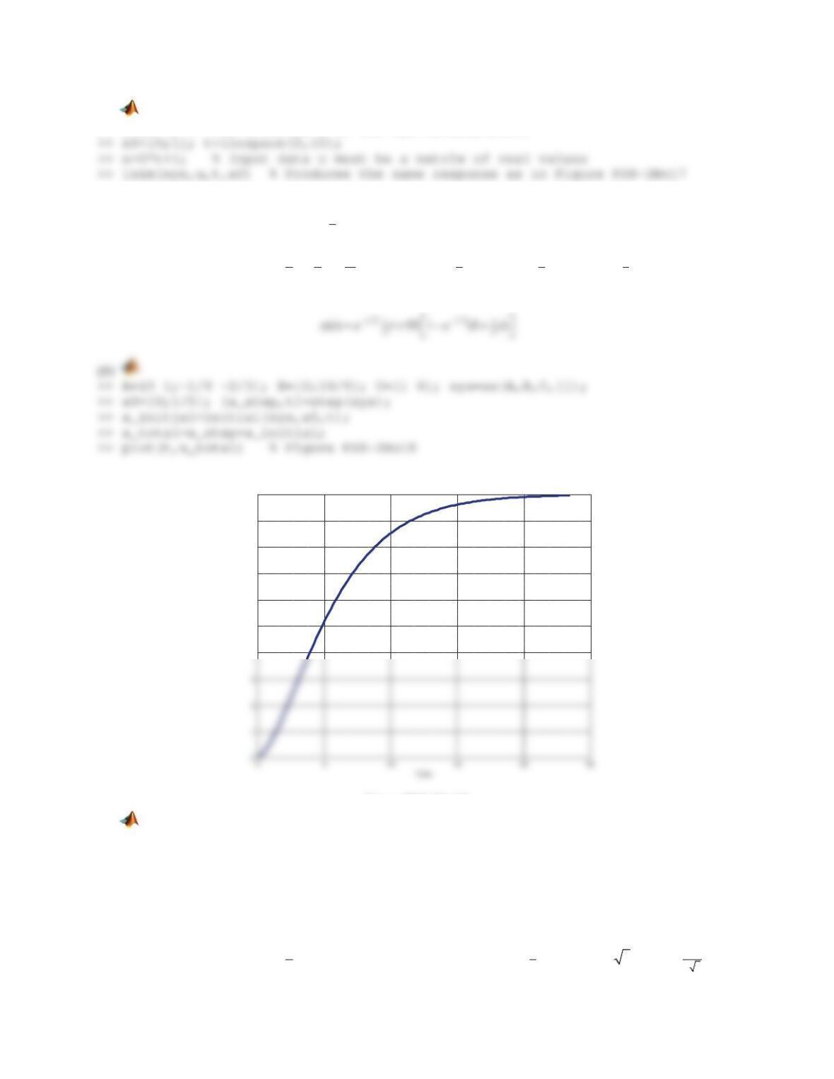
2. Consider a first-order system with time constant
W
and zero initial condition. Find the system’s unit-step
response for 1
3
W
and 2
3
W
, plot the two curves versus
02tdd
in the same graph, and comment.
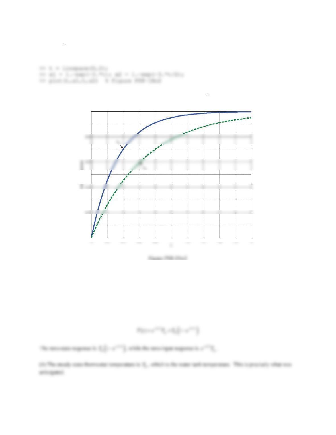
Solution
When 1
3
W
, the unit-step response is
00.2 0.4 0.6 0.8 11.2 1.4 1.6 1.8 2
0
0.5
2.5
3
3.5
4
312
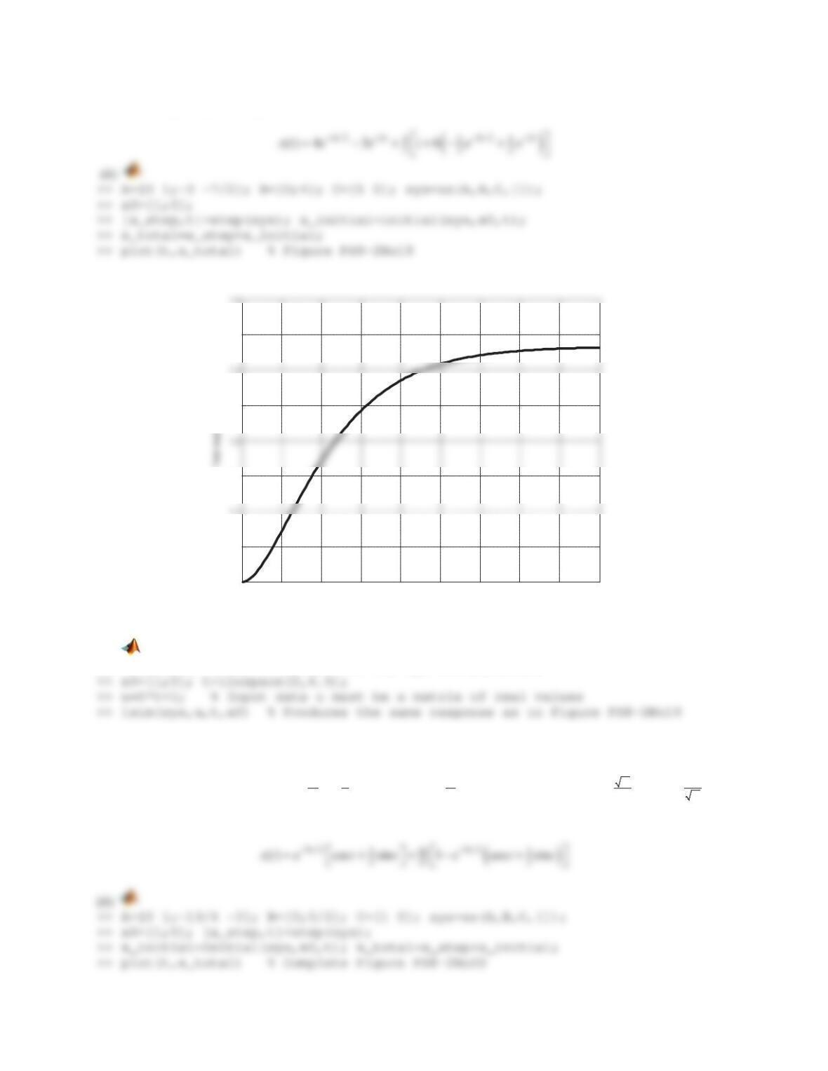
When 2
3
W
, it is
3/2
2
() 1
t
xt e
As expected, the response
1
x
associated with the smaller time constant 1
3
W
reaches steady-state faster.
3. A thermostat, initially at ambient temperature
(0)
a
TT
, is placed inside a water tank whose temperature is
fixed at b
T. The thermostat temperature is the response of
b
TT T
W
where
const
W
depends on thermal
resistance and capacitance.
(a) Find the zero-state and zero-input responses.
(b) Find the steady-state thermostat temperature.
Solution
(a) The input is a step function with magnitude b
T. Therefore, the response is
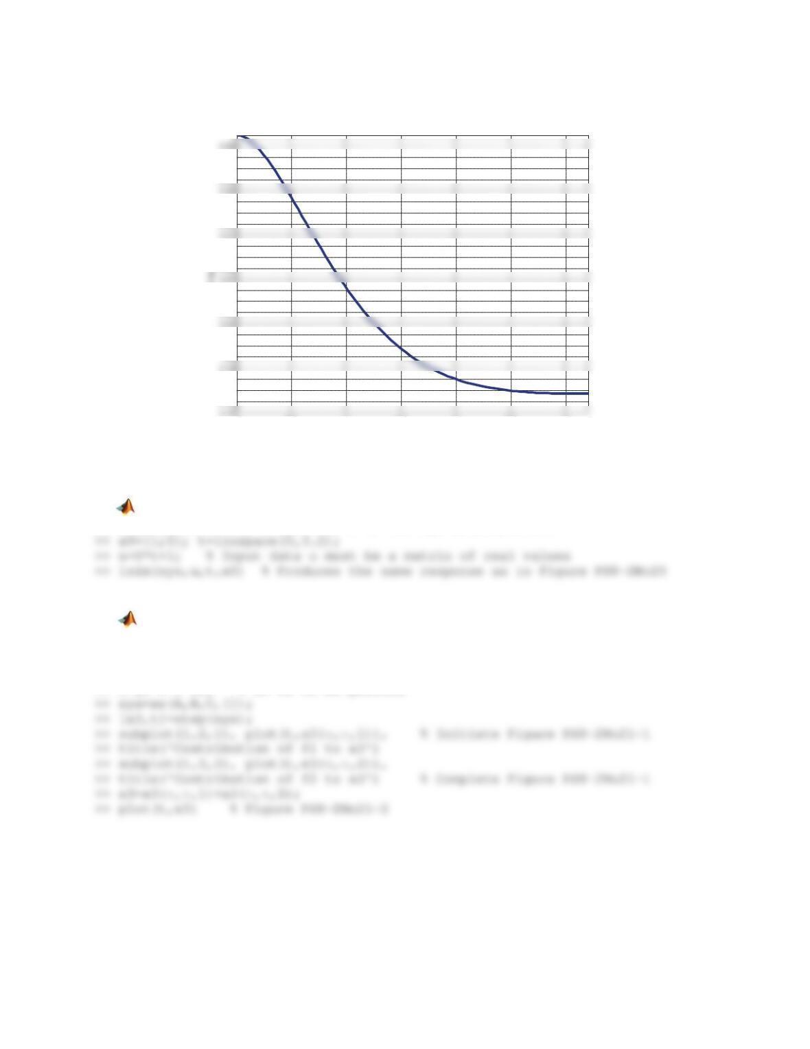
4. Repeat Problem 3 for the case when the temperature of the water tank increases linearly with time at a rate of
r
00.2 0.4 0.6 0.8 11.2 1.4 1.6 1.8 2
0
0.1
0.3
0.5
0.7
0.9
1
313
.
Solution
(a)
TT rt
W
. The input is a ramp function with magnitude
r
, hence the response is
5. A single-tank liquid-level system with inflow rate
i
q
as its input and liquid level
h
as its output is modeled as
(), (0) 0
i
RAh gh Rq t h
, where
,,R A g const
. If the inflow rate is a unit-step, find the system response
in terms of the physical parameters. Also find the steady-state response.
Solution
Rewriting the model in standard form, we find
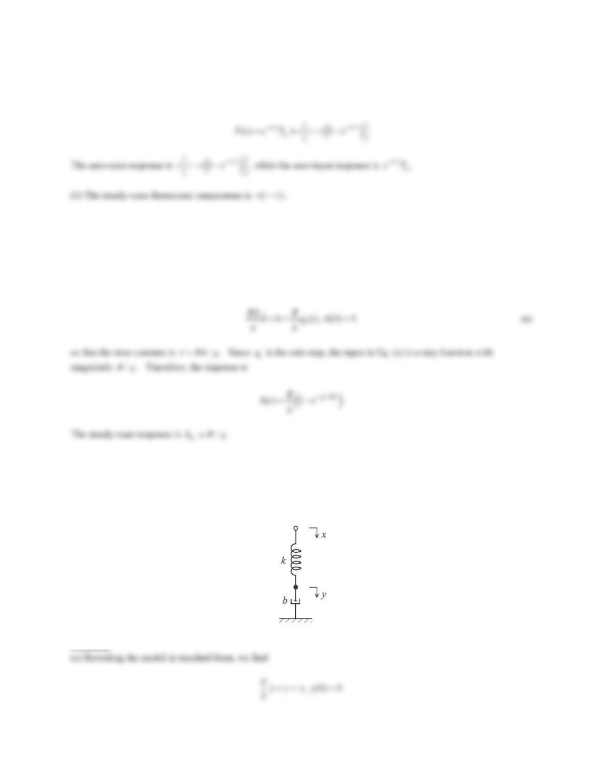
6. The equation of motion of the mechanical system is Figure 8.4 is
()0by k y x
where
x
and
y
are the
input and the output, respectively, and
,b k const
. Assuming zero initial condition, find the response when
x
is a
(a) unit-step,
(b) unit-ramp.
Figure 8.4 Problem 6.
314
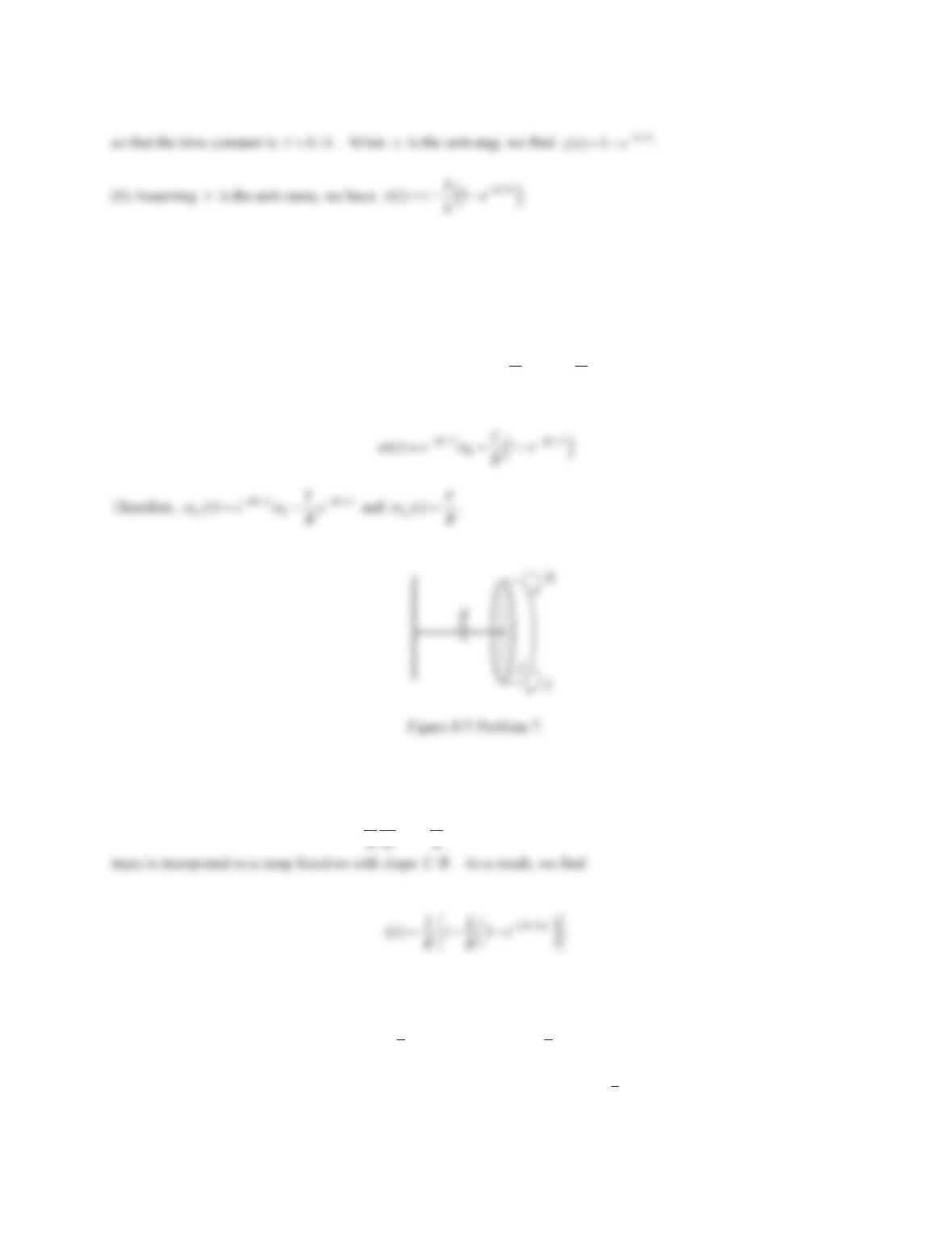
7. The torsional mechanical system in Figure 8.5 is modeled as
()JBTt
TT
, where
,J B const
,
T
is the
angular displacement, and
T
is a constant applied torque. Rewrite the model as first-order in angular velocity
ZT
. Assuming
0
(0)
ZZ
, determine ()t
Z
. Also identify the transient and steady-state responses.
Solution
The model is expressed as
JBT
ZZ
, and in standard form
JT
BB
ZZ
so that the time constant is
/JB
W
.
Since T const , the input is interpreted as a step function with magnitude
/TB
, and
8. Find the unit-ramp response of the RL circuit in Example 8.3.
Solution
The governing equation of the circuit is
1()
a
Ldi ivt
where
ar
vu
. The time constant is
/LR
W
and the
9. A first-order dynamic system is modeled as
12
23
5 ( ) , (0)vvFtv
Find the response
()vt
if the input
()Ft
is a ramp function with a slope of 3
2. Also find the steady-state
response and the steady-state error.
315
Solution
In standard form, we have
11
10 5
()vv Ft
so that 1
10
W
and the input is interpreted as a ramp of slope
3
10
.The
response is
10. A first-order dynamic system is modeled as
3 ( ) , (0) 1wwgtw
Find ()wt if the input
()gt
is a step function with magnitude
10
. Also find
ss
w
. How many time units will it
take for the response curve to reach within 2% of
ss
w
?
Solution
In standard form, we have
11
33
()ww gt
so that 1
3
W
and the input is interpreted as a step of magnitude
10
3
. The
response is
Problem Set 8.2
1. Show that the free response of an overdamped, second-order system stabilizes at zero after a sufficiently long
time.
Solution
In this case, the two poles are given by 2
11
nn
s
]Z Z ]
,
2
21
nn
s
]Z Z ]
. Since
21
]]
, we
In Problems 2 through 6, for each given system model,
(a) Identify the damping type and find the free response.
(b) Find and plot the free response using the initial command.
2.
2 2 0 , (0) 0 , (0) 1xxx x x
Solution
(a) In standard form,
1
implies
21
Z
and 21
]Z
. Therefore, 1
Z
and
1
]
, hence the
316
(b)
>> A=[0 1;-1/2 -1]; C=[1 0]; sys=ss(A,[],C,[]);
3.
3 9 0 , (0) 1 , (0) 0xxx x x
Solution
(a) Comparing with the standard form, we find
2
9
n
Z
and
23
n
]Z
. Therefore,
3 r/s
n
Z
and
1
2
]
, hence the
0.2
0.4
0.6
0.7
Response to Initial Conditions
00.5 11.5 22.5 33.5 4
0
0.2
0.6
1
1.2
Response to Initial Conditions
Time (seconds)
317
4.
1
2
2 5 3 0 , (0) , (0) 1xxx x x
Solution
(a) Comparing 53
220xxx
with the standard form, we find
23
2
n
Z
and
5
2
2n
]Z
. Therefore, 3
2 r/s
n
Z
5.
4 4 0 , (0) 1 , (0) 1xxx x x
Solution
(a) Comparing
1
4
0xx x
with the standard form, we find
21
4
n
Z
and 21
n
]Z
. Therefore,
1
2
r/s
n
Z
and
1
]
, hence the system is critically damped. Therefore
0.1
0.2
0.4
0.6
0.8
Response to Initial Conditions
Amplitude
318
6.
4 4 5 0 , (0) 0 , (0) 1xxx x x
Solution
(a) Comparing 5
40xx x
with the standard form, we find
25
4
n
Z
and 21
n
]Z
. Therefore,
5
2 r/s
n
Z
and
Figure PS8-2No6
7. Show that the impulse response of an underdamped, second-order system stabilizes at zero after a sufficiently
long time.
Solution
The impulse response is given as
00
0
() cos sin
ntn
dd
d
xxA
xt e x t t
]Z
]Z
ZZ
Z
ªº
«»
¬¼
0.2
0.4
0.8
1.4
1.6
Response to Initial Conditions
Amplitude
02 4 6 8 10 12
-0.2
0
0.1
0.3
0.5
0.6
Respons e to Initial Conditions
Time (seconds)
319
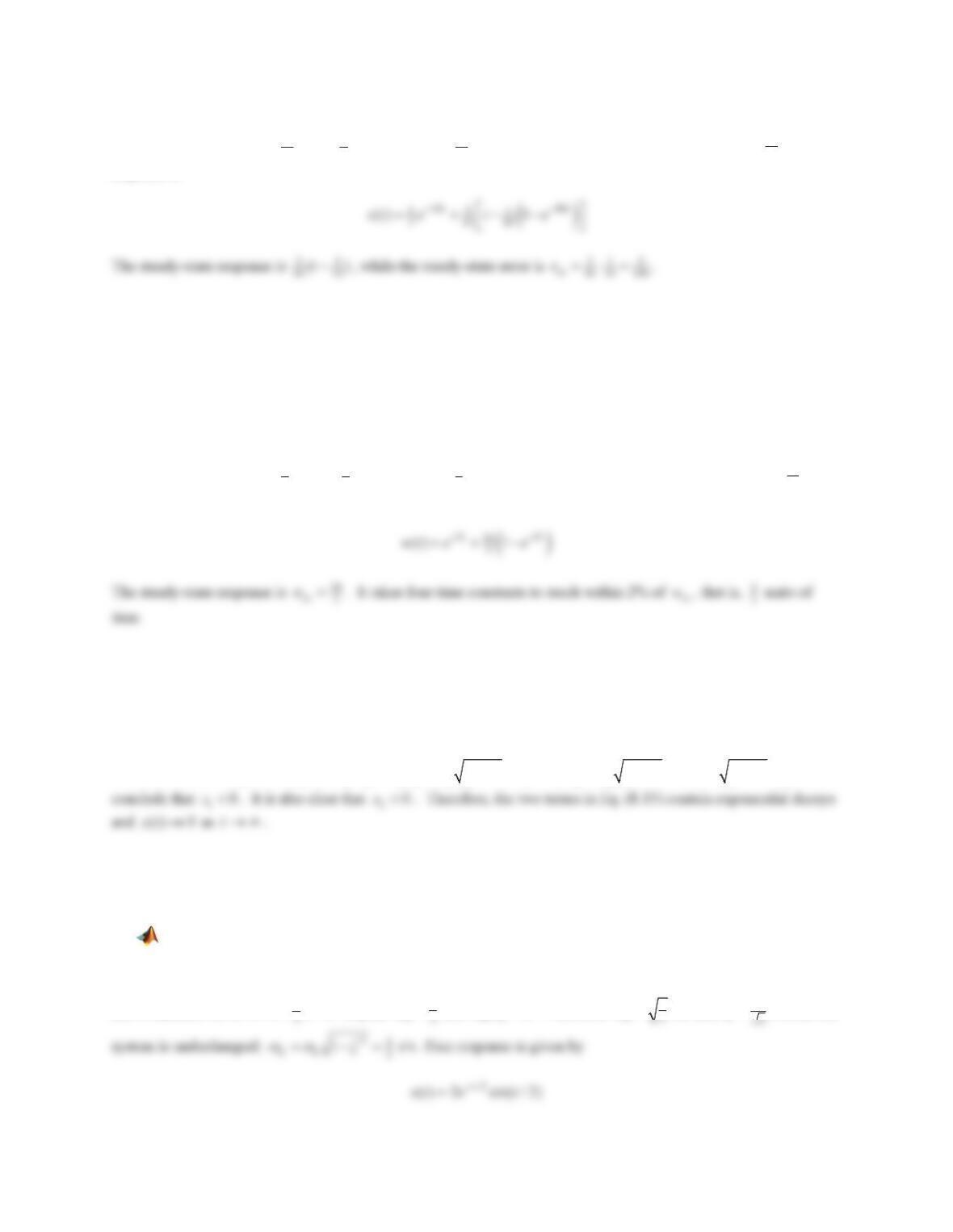
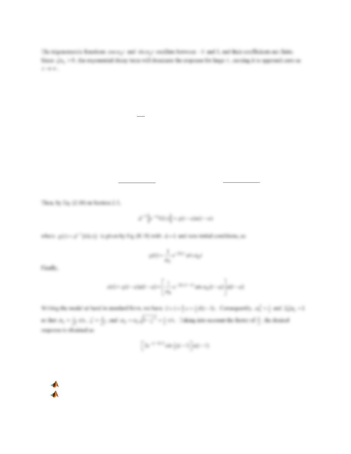
8. Show that the response of an underdamped, second-order system to an impulsive input
()ta
G
,
0a const !
,
and zero initial conditions, is described by
()
1sin ( ) ( )
nta
d
d
etauta
]Z Z
Z
ªº
«»
¬¼
where
()ut
is the unit-step function. Use this result to find the response
()xt
of
2 2 ( 1) , (0) 0 , (0) 0xxx t x x
G
Solution
Recalling
{( )}
as
ta e
G
L
, the response under consideration is provided by
^`
11
22
() ( )
()
as
as
nd
e
xt e Gs
s
]Z Z
½
°°
®¾
°°
¯¿
LL
,
22
1
() ()
nd
Gs s
]Z Z
In Problems 9 and 10, assuming zero initial conditions,
(a) Find the response
()xt
in closed form.
(b) Plot the response using the impulse command.
(c) Plot the response through the simulation of the Simulink model of the system.
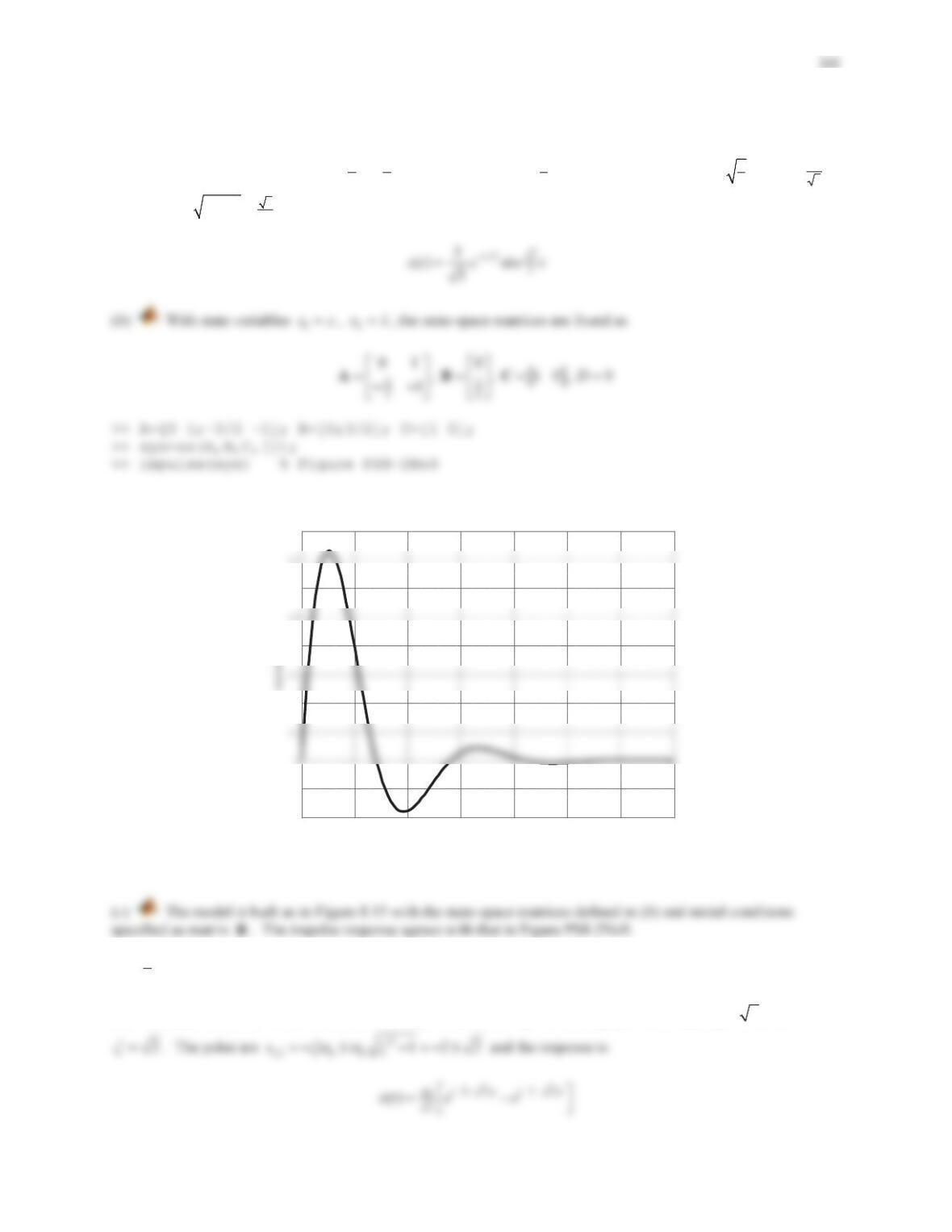
9.
2233()xxx t
G
Solution
(a) In standard form, we have
33
22
()xx x t
G
. Therefore,
23
2
n
Z
and 21
n
]Z
so that 3
2 r/s
n
Z
,
1
6
]
,
and
25
2
1 r/s
dn
ZZ ]
. The response is
Figure PS8-2No9
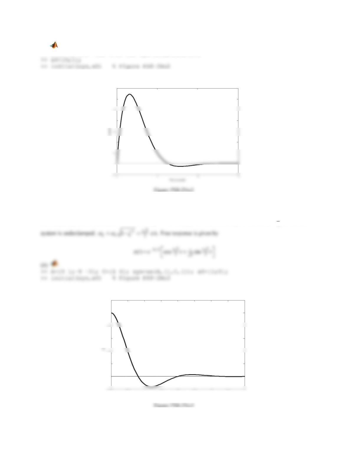
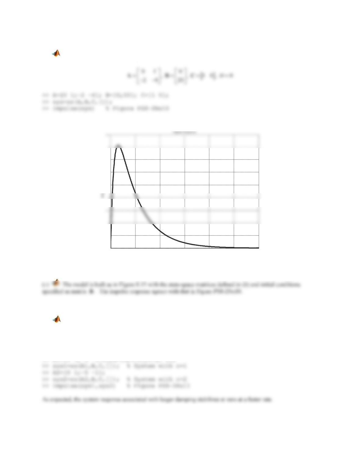
10.
1
2210()xxx t
G
Solution
(a) In standard form, we have 42 20()xxx t
G
. Therefore,
2
2
n
Z
and
24
n
]Z
so that
2 r/s
n
Z
,
0 2 4 6 8 10 12 14
-0.2
-0.1
0.2
0.4
0.6
0.8
Impulse Response
Time (seconds)
321
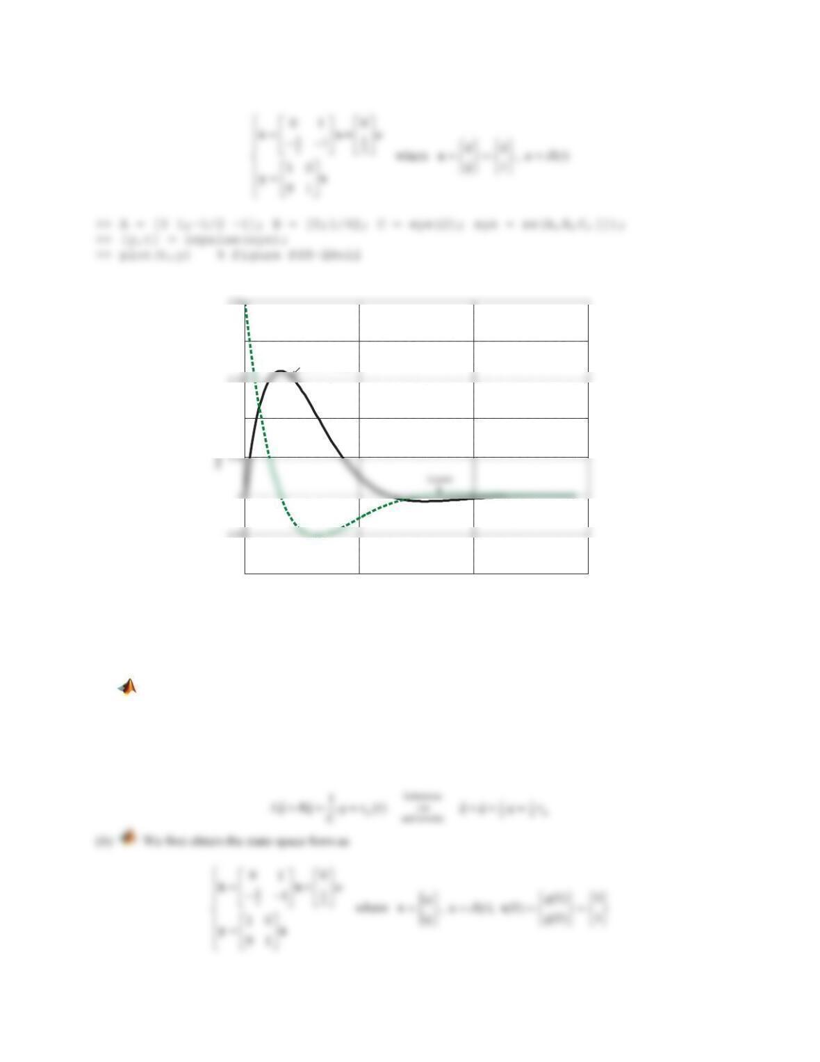
(b) With state variables
1
xx
,
2
xx
, the state-space matrices are found as
Figure PS8-2No10
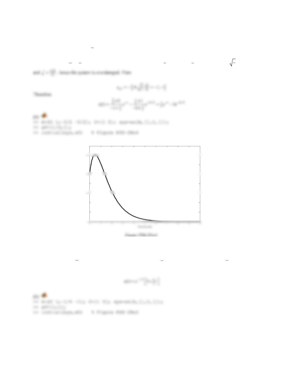
11. Consider a mass-spring-damper system as in Figure 8.6 of this section, where
2 kg , 10 N/mmk
Assuming zero initial conditions, plot (in a single figure) the response
x
to a unit-impulse force for two cases
of
1 N-sec/mc
and
2 N-sec/mc
, and discuss the results.
Solution
0 2 4 6 8 10 12
0
0.5
2.5
3
3.5
Time (seconds)
322
Figure PS8-2No11
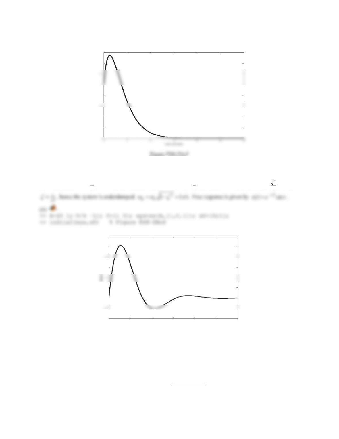
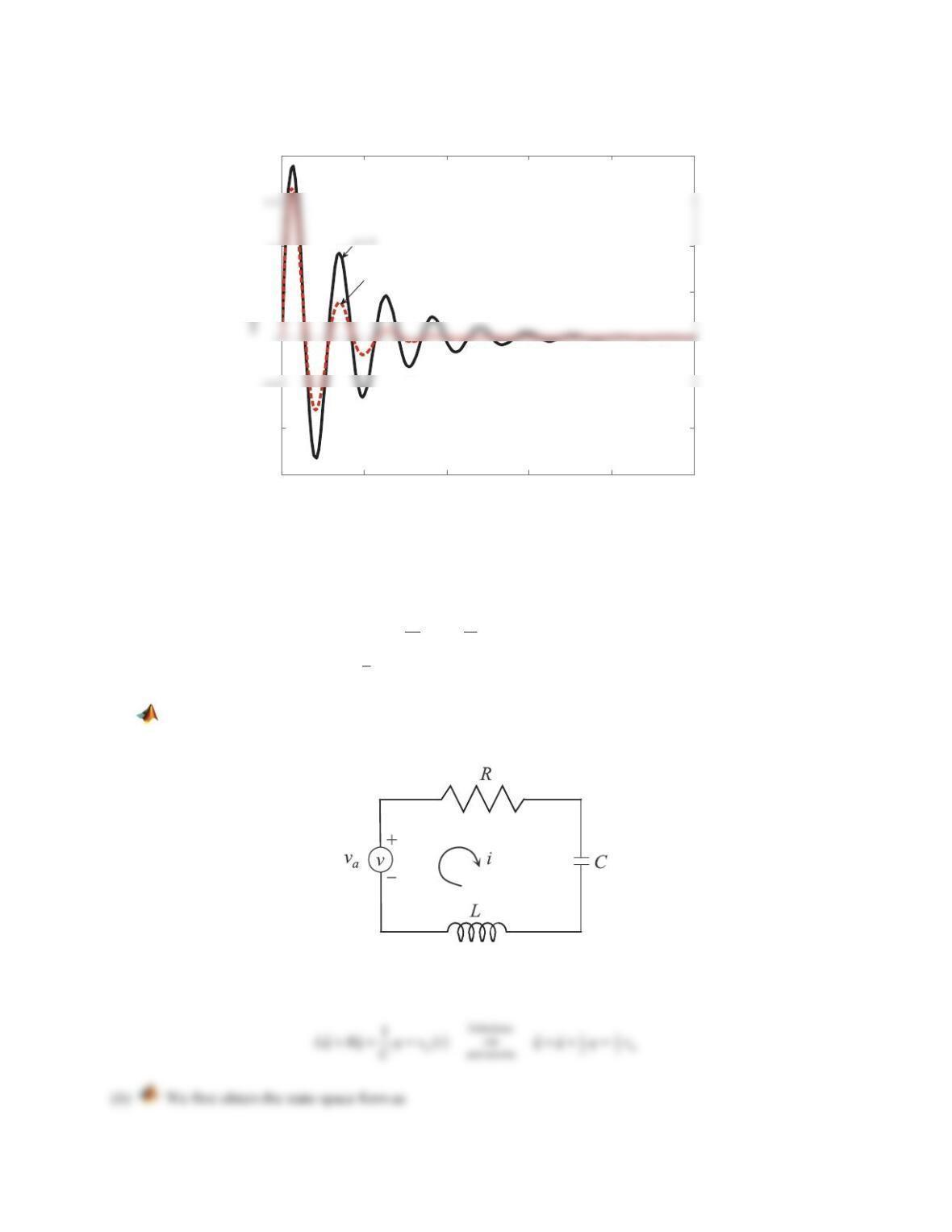
12. The governing equation for the RLC circuit in Figure 8.20 is derived as
1 ()
a
di
LRi idtvt
dt C
³
where
4 HL
,
4R :
and
1
2 FC
.
(a) Write the governing equation in terms of the electric charge q, where
iq
.
(b) Plot qand
i
versus
t
(same figure) when the applied voltage a
vis a unit-impulse and initial conditions
are zero.
Figure 8.20 Problem 12.
Solution
(a) Using
iq
, the governing equation is expressed as
0 5 10 15 20 25
-0.15
-0.1
0.05
0.1
0.2
Impulse Response
Time (seconds)
c = 2
323
Figure PS8-2No12
13. Consider the RLC circuit in Problem 12.
(a) Write the governing equation in terms of the electric charge q, where
iq
.
(b) Plot qand
i
versus
t
(same figure) when the applied voltage a
vis a unit-impulse and initial conditions
are (0) 0q ,
(0) 1q
.Hint: Find the superposition of the data returned by impulse and initial
commands.
Solution
(a) Using
iq
, the governing equation is expressed as
0 5 10 15
-0.1
0.1
0.2
Time (sec)
Electric charge
324
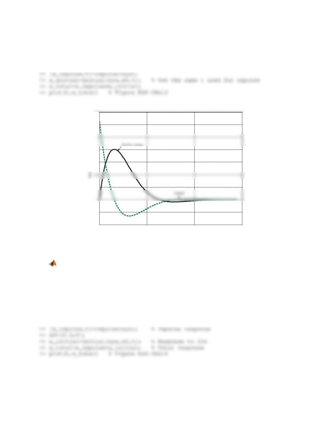
>> A = [0 1;-1/2 -1]; B = [0;1/4]; C = eye(2);
>> x0=[0;1];
>> sys=ss(A,B,C,[]);
Figure PS8-2No13
14. Consider a mass-spring-damper system as in Figure 8.6 of this section, where
3 kg , 2 N-sec/m, 10 N/mmc k
Plot (in a single figure) the responses
x
and x
to a unit-impulse force and initial conditions
(0) 0.3x
,
(0) 0x
.
Solution
>> A = [0 1;-10/3 -2/3]; B = [0;1/3]; C = eye(2);
>> sys=ss(A,B,C,[]);
0 5 10 15
-0.4
-0.2
0.2
0.6
0.8
1.2
1.4
Time
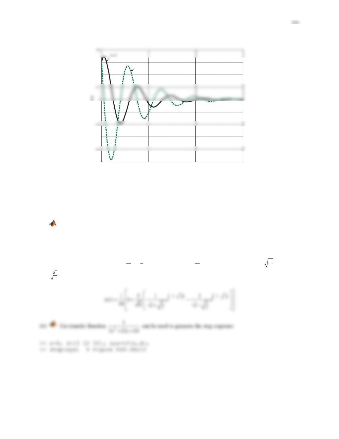
Figure PS8-2No14
In Problems 15 and 16,
()ut
denotes the unit-step. Assuming zero initial conditions,
(a) Find the response
()xt
in closed form.
(b) Plot the response using the step command.
15.
31210 ()xxxut
Solution
(a) In standard form, we have
10 1
33
4()xx x ut
. Therefore,
210
3
n
Z
and
24
n
]Z
so that 10
3 r/s
n
Z
,
23
10
1
]
!
. The (overdamped) system response is
0 5 10 15
-0.5
-0.3
-0.1
0.2
0.3
Time
Total response
x
2
=xdot
326
Figure PS8-2No15
16.
25
8
23 5()xx xut
Solution
(a) In standard form, we have
325 5
216 2
()xx xut
. Therefore,
225
16
n
Z
and
3
2
2n
]Z
so that 5
4 r/s
n
Z
,
0123456
0
0.01
0.02
0.04
0.06
0.08
0.1
Step Response
Time (seconds)
0
0.2
0.4
0.8
1.2
1.6
327
In Problems 17 through 20,
()ut
denotes the unit-step. Given the non-zero initial conditions,
(a) Find the response
()xt
in closed form.
(b) Plot the response using the step and initial commands.
(c) Plot the response using lsim.
17.4 3 ( ), (0) 0, (0) 1xx x utx x
Solution
(a) Comparing with the standard form, we have
2
4
n
Z
and 21
n
]Z
so that
2 r/s
n
Z
,
1
4
1
]
, and
15
2 r/s
d
Z
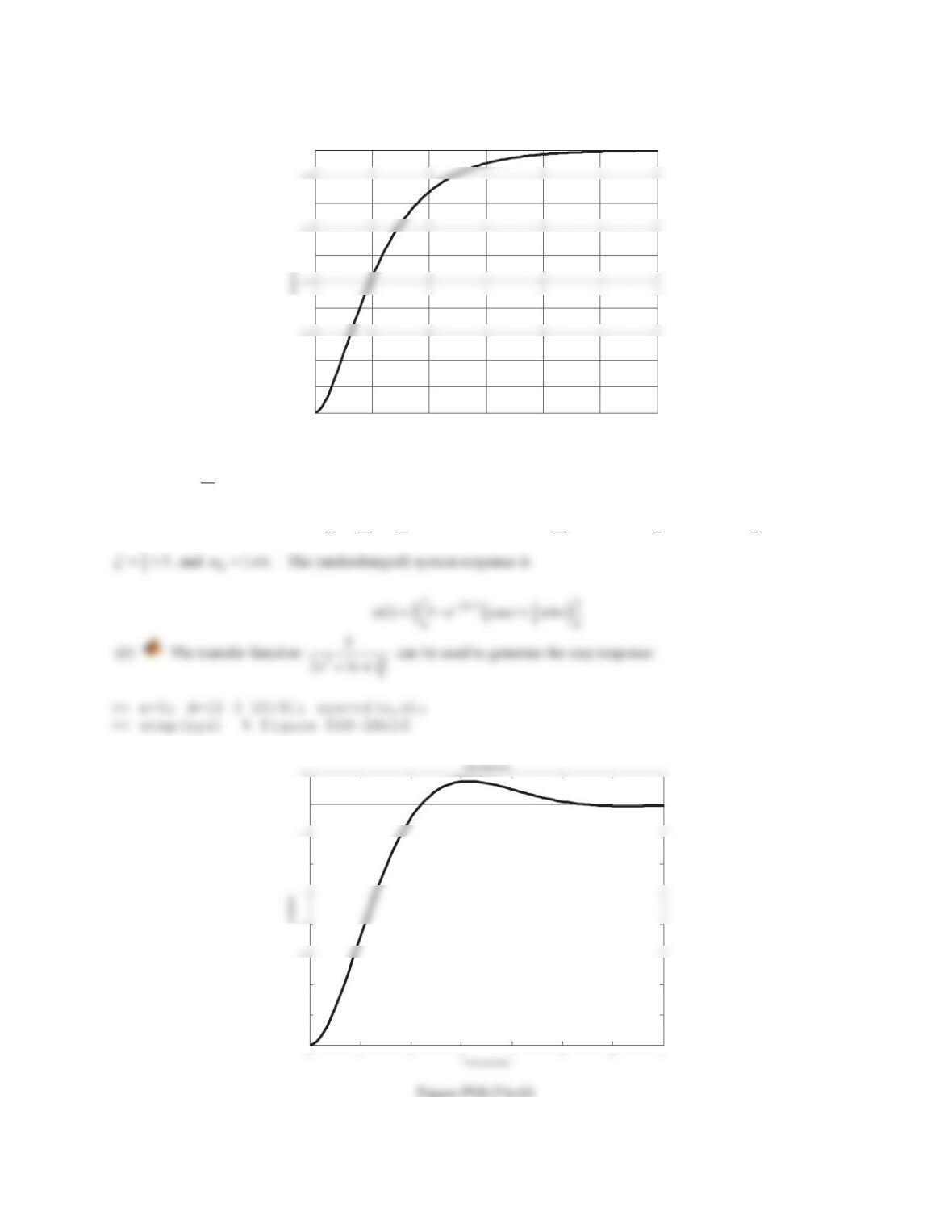
. The (underdamped) system response is
(b)
>> A=[0 1;-4 -1]; B=[0;3]; C=[1 0]; sys=ss(A,B,C,[]);
>> x0=[0;1]; [x_step,t]=step(sys);
>> x_initial=initial(sys,x0,t);
Figure PS8-2No17
0 1 2 3 4 5 6 7 8 9 10
-0.2
0
0.2
0.6
1
1.2
Total response
Step response
328
(c)
>> A=[0 1;-4 -1]; B=[0;3]; C=[1 0]; sys=ss(A,B,C,[]);
18.
1
5
9 6 10 ( ), (0) 0, (0)xxx utx x
Solution
(a) In standard form, we have
10
21
39 9
()xxx ut
so that
21
9
n
Z
and
2
3
2n
]Z
so that
1
3 r/s
n
Z
,
1
]
. The
(critically damped) system response is
Figure PS8-2No18
(c)
>> A=[0 1;-1/9 -2/3]; B=[0;10/9]; C=[1 0]; sys=ss(A,B,C,[]);
>> x0=[0;1/5]; t=linspace(0,25);
>> u=0*t+1; % Input data u must be a matrix of real values
>> lsim(sys,u,t,x0) % Produces the same response as in Figure PS8-2No18
19.
2 7 6 8 ( ), (0) 1, (0) 0xxxutx x
Solution
(a) In standard form, we have
7
2
34()xxxut
so that
2
3
n
Z
and
7
2
2n
]Z
so that
3 r/s
n
Z
,7
43 1
]
!
.
4
5
6
7
8
9
10
Total response
329
The (overdamped) system response is
Figure PS8-2No19
(c)
>> A=[0 1;-3 -7/2]; B=[0;4]; C=[1 0]; sys=ss(A,B,C,[]);
20.
4 12 13 10 ( ), (0) 1, (0) 0xxxutx x
Solution
(a) In standard form, we have 13 5
42
3()xx x ut
so that
213
4
n
Z
and
23
n
]Z
so that
13
2 r/s
n
Z
,
3
13 1
]
,
and 1 r/s
d
Z
. The (underdamped) system response is
00.5 11.5 22.5 33.5 44.5
1
1.05
1.15
1.25
1.35
Time
330
Figure PS8-2No20
(c)
>> A=[0 1;-13/4 -3]; B=[0;5/2]; C=[1 0]; sys=ss(A,B,C,[]);
21. Repeat Example 8.9 when
1
x
is the output.
Solution
>> A=[0 0 1 0;0 0 0 1;-2 1 -1 1;1/2 -1/2 1/2 -1/2];
>> B=[0 0;0 0;1 0;0 1/2];
>> C=[0 0 1 0]; % x3 is to be plotted
00.5 11.5 22.5 3
0.76
0.77
0.78
0.8
0.81
0.82
0.84
0.85
0.86
0.88
0.89
0.9
0.92
0.93
0.94
0.97
0.98
Time
Total response


