Unlock document.
This document is partially blurred.
Unlock all pages and 1 million more documents.
Get Access
194
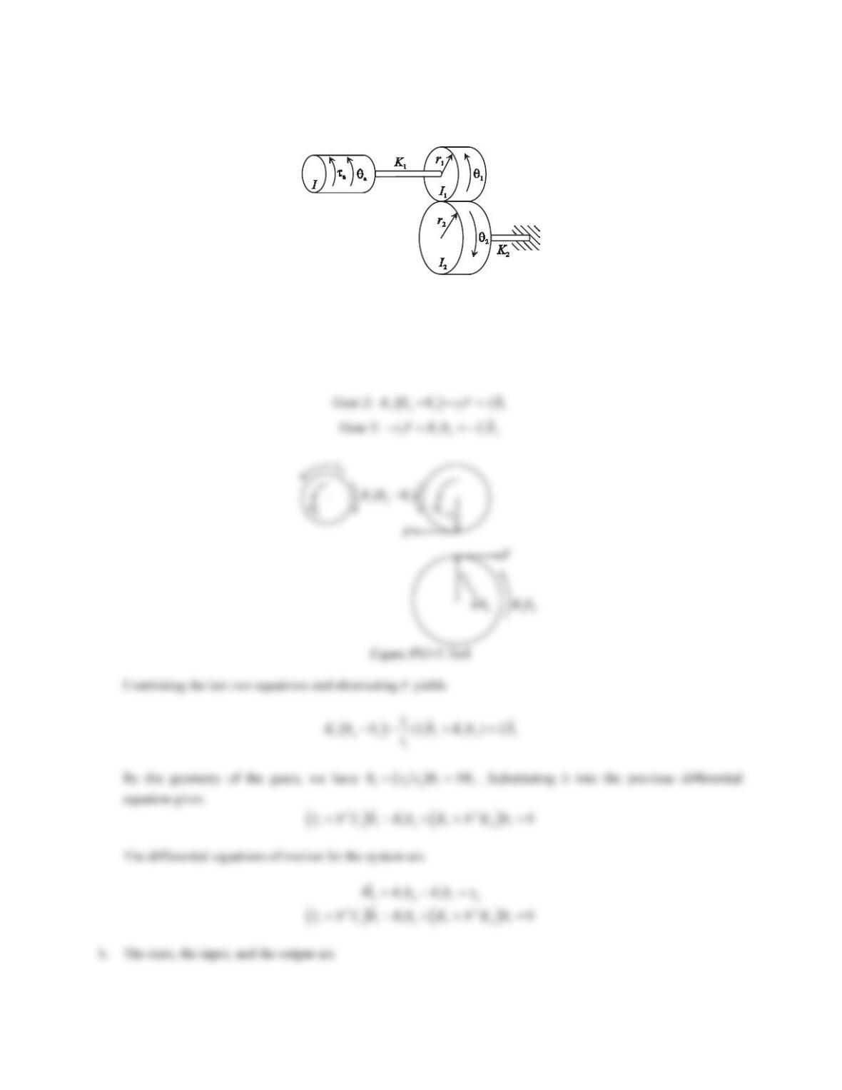
b. Using the differential equation obtained in Part (a), determine the state-VSDFHUHSUHVHQWDWLRQ8VHșa,ș1Ȧa,
DQGȦ1as tKHVWDWHYDULDEOHVDQGXVHș2DQGȦ2as the output variables.
Figure 5.99 Problem 4.
Solution
a. Assume that a1
șș!!
. The free-body diagram is shown below. Applying the moment equation to each gear,
+ր:
OO
ĮMI¦
Gear 1:
a1a1 a
șș șKI
W
195
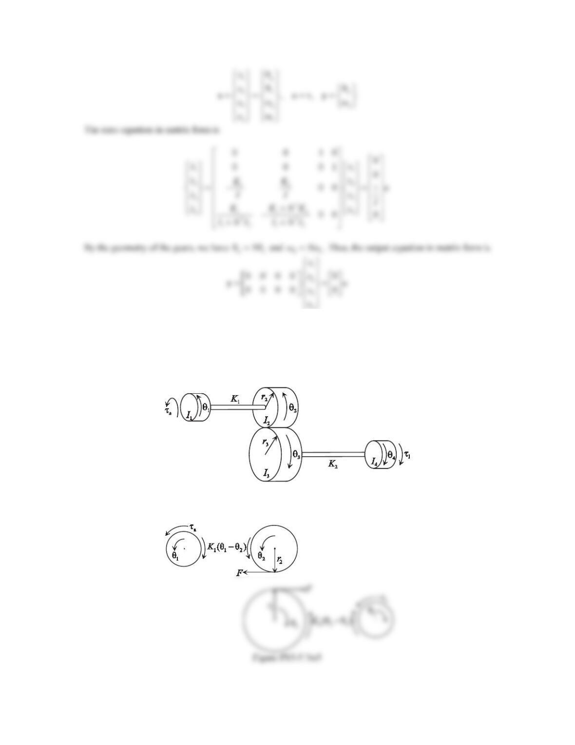
5. A three-degree-of-freedom gear–train system is shown in Figure 5.100, which consists of four gears of
moments of inertia I1,I2,I3, and I4. Gears 2 and 3 are meshed and their radii are r2and r3, respectively. Gears 1
and 2 are connected by a relatively long shaft, and gears 3 and 4 are connected in the same way. The shafts are
DVVXPHGWREHIOH[LEOHDQGFDQEHDSSUR[LPDWHGE\WRUVLRQDOVSULQJV7KHDSSOLHGWRUTXHDQGORDGWRUTXHDUHIJa
DQGIJlon gear 1 and gear 4, respectively. The gears are assumed to be rigid and have no backlash. Derive the
differential equations of motion.
Figure 5.100 Problem 5.
Solution
Assume that
12
șș !!
and
34
șș!!
. The free-body diagram is shown in the figure below.
196
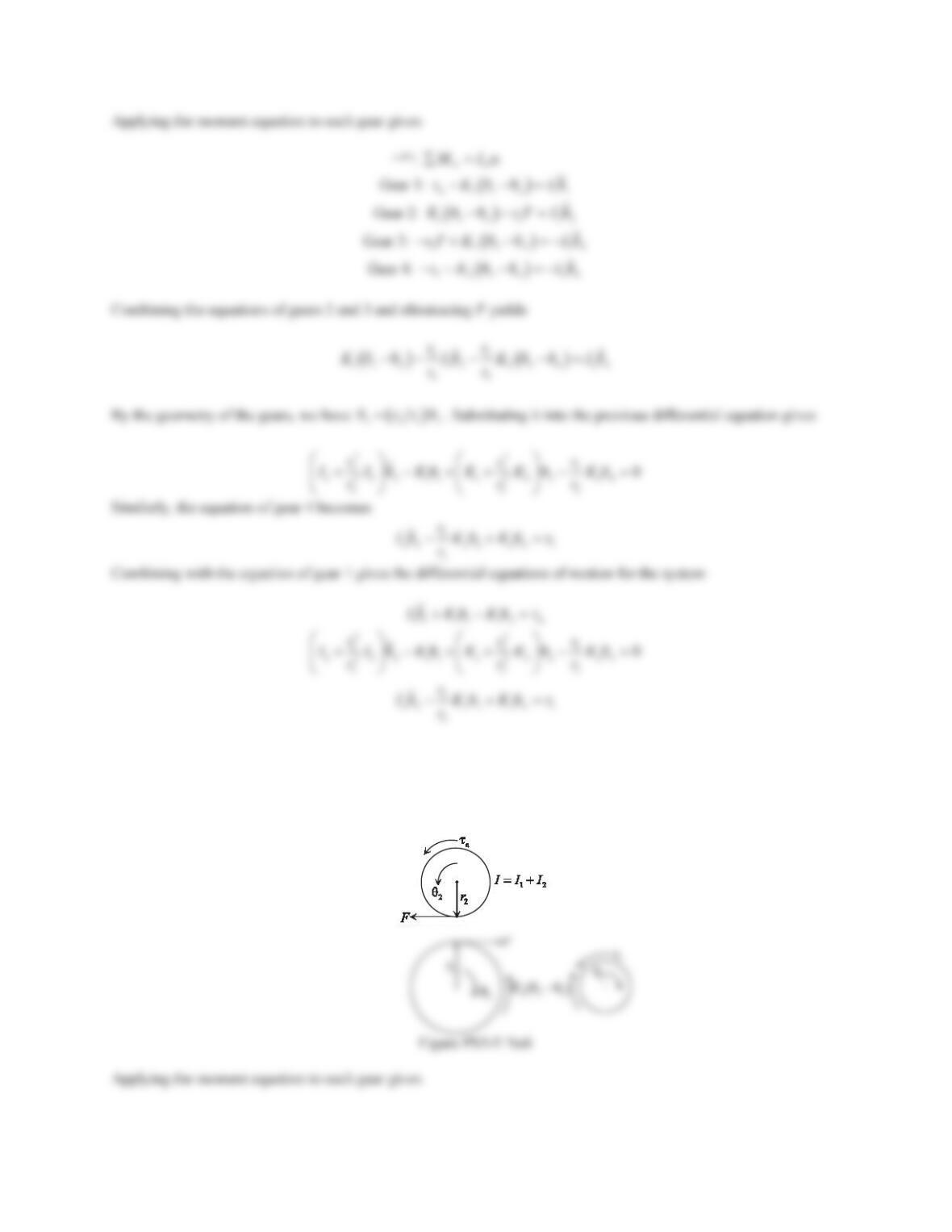
6. Repeat Problem 5. Assume that the shaft connecting gears 1 and 2 is relatively short and rigid.
Solution
Assume that the shaft connecting gears 1 and 2 is relatively short and rigid, we have
12
șș
. Assume that
34
șș!!
. The free-body diagram is shown in the figure below.
197
Problem Set 5.6
(Note: All MATLAB figures are given at the end of Problem Set 5.6.)
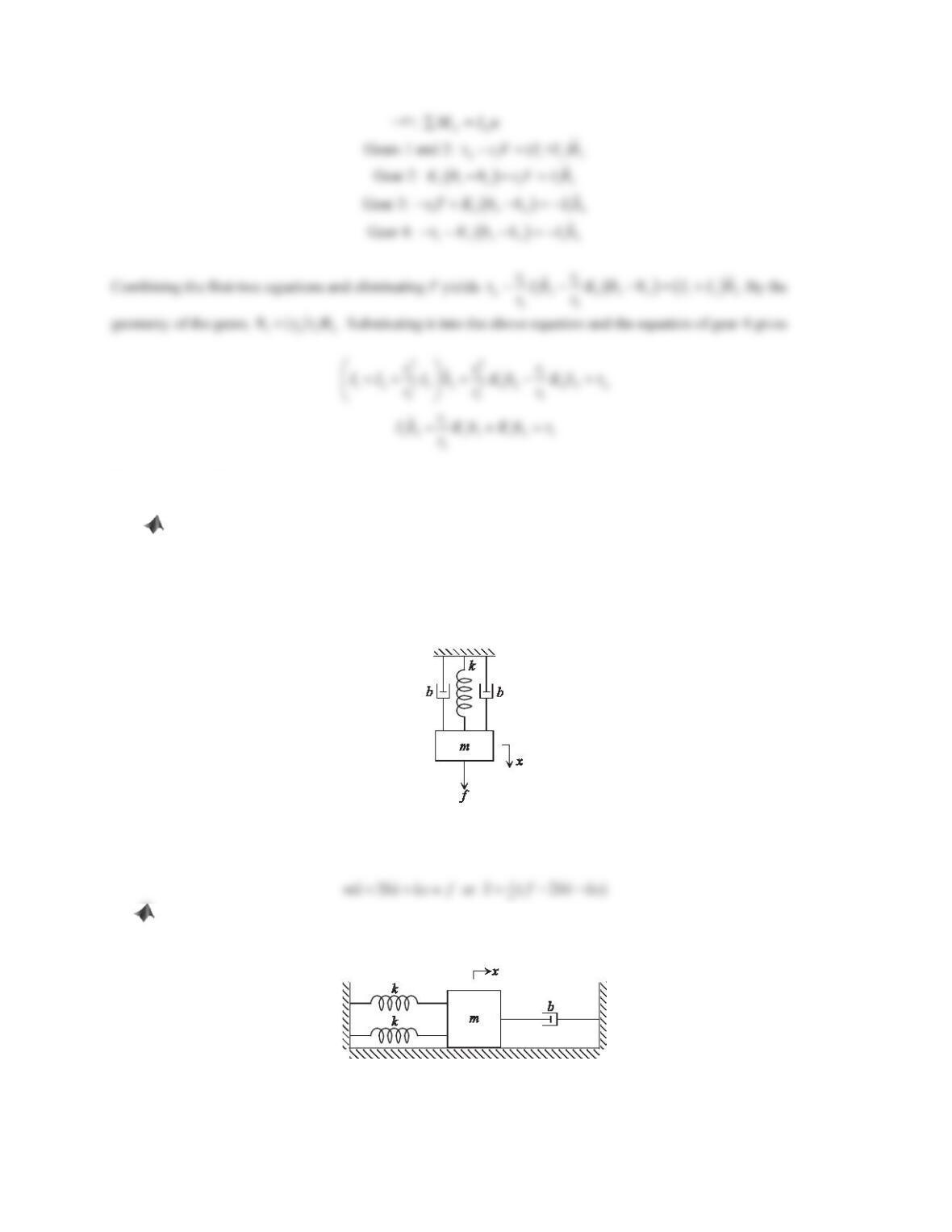
1. Consider the mass–spring–damper system shown in Figure 5.116, where the force acting on the mass
block is a unit-impulse function with a magnitude of 10 N and a duration of 0.1 sec. The parameter values are m
= 25 kg, b= 20 Ns/m, and k= 100 N/m.
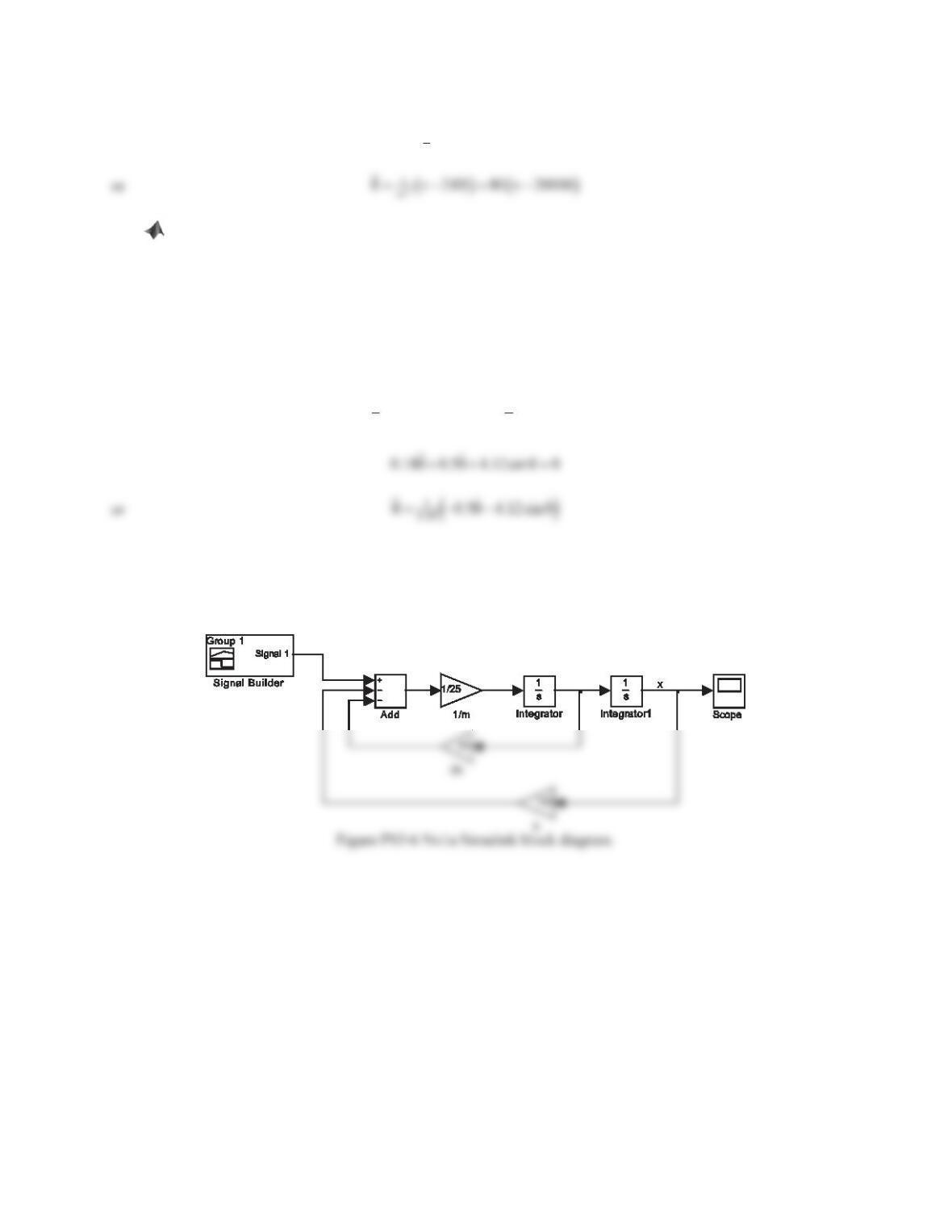
a. Build a Simulink model based on the differential equation of motion of the system and find the
displacement output x(t).
b. Build a Simscape model of the physical system and find the displacement output x(t).
Figure 5.116 Problem 1.
Solution
The differential equation of the system is
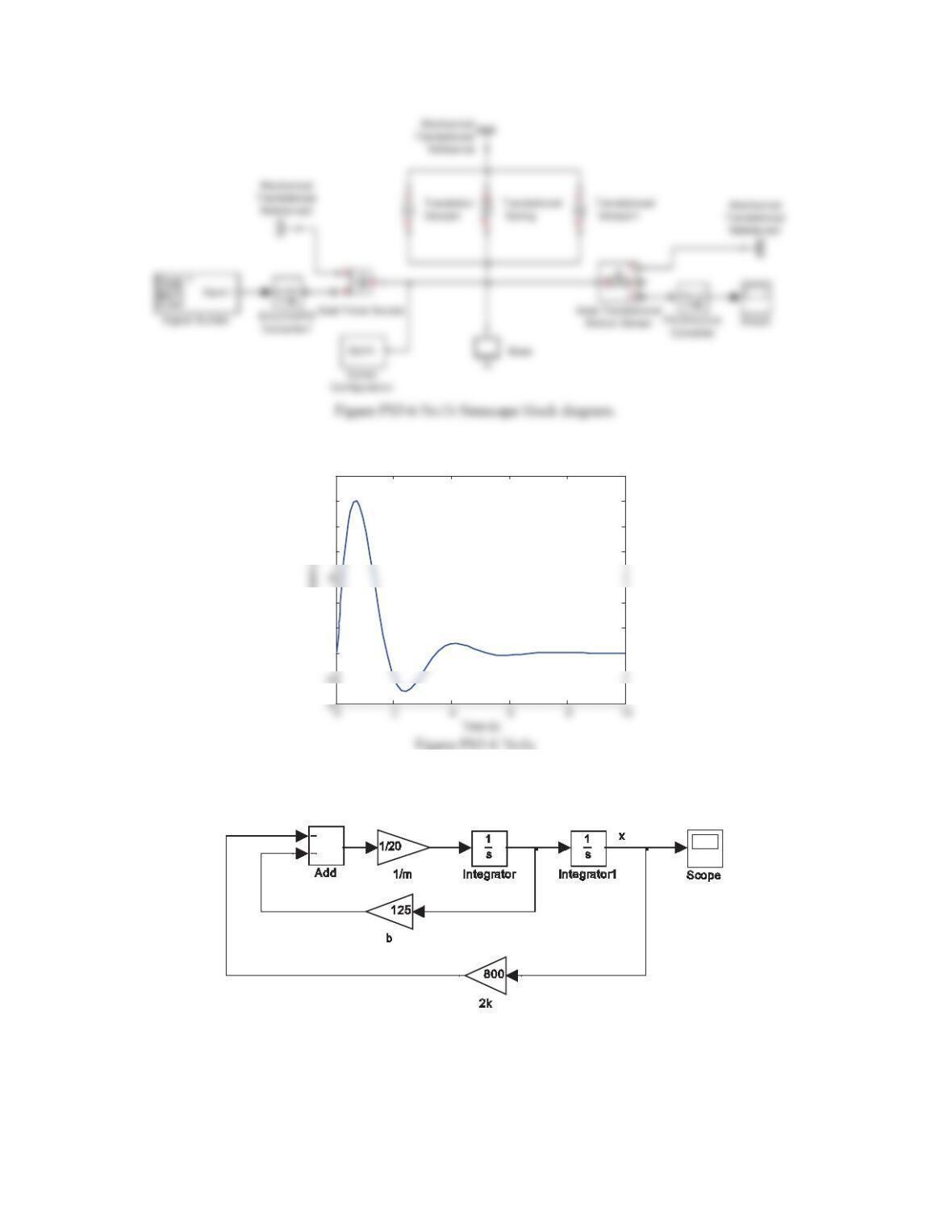
2. Repeat Problem 1 for the mass–spring–damper system shown in Figure 5.117, where the origin of the
coordinate xis set at equilibrium. Assume x(0) = 0.1 m and
(0) 0x
m/s. The parameter values are m= 20 kg,
b= 125 Ns/m, and k= 400 N/m.
Figure 5.117 Problem 2.
Solution
The differential equation of the system is
198
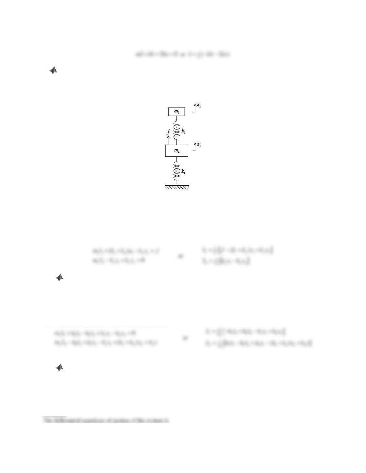
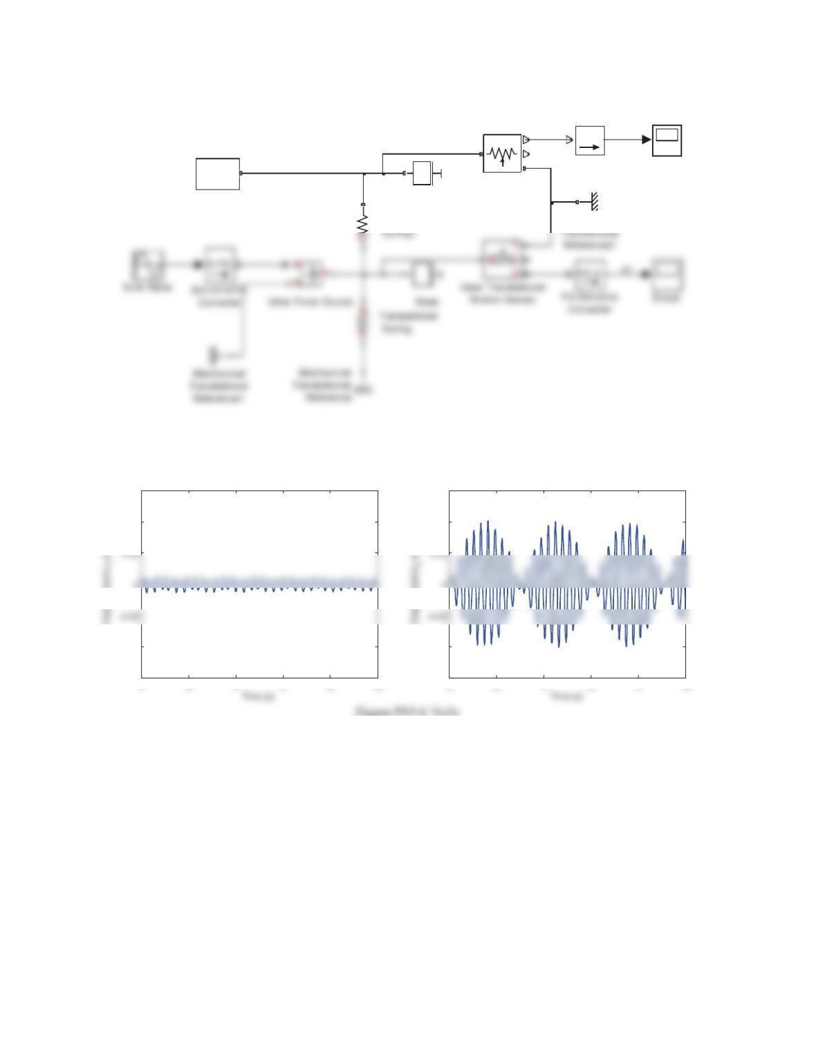
3. Consider the mass–spring–damper system shown in Figure 5.118. The mass block m1and the spring k1
represent a rotating machine, which is subjected to a harmonic disturbance force f= 40sin(7St) N due to a rotating
unbalanced mass. The mass block m2and the spring k2represent a vibration absorber (see Section 9.3 for more
details), which is designed to reduce the displacement of the machine. The parameter values are m1= 6 kg, k1= 6000
N/m, m2= 1.65 kg, and k2= 800 N/m.
Figure 5.118 Problem 3.
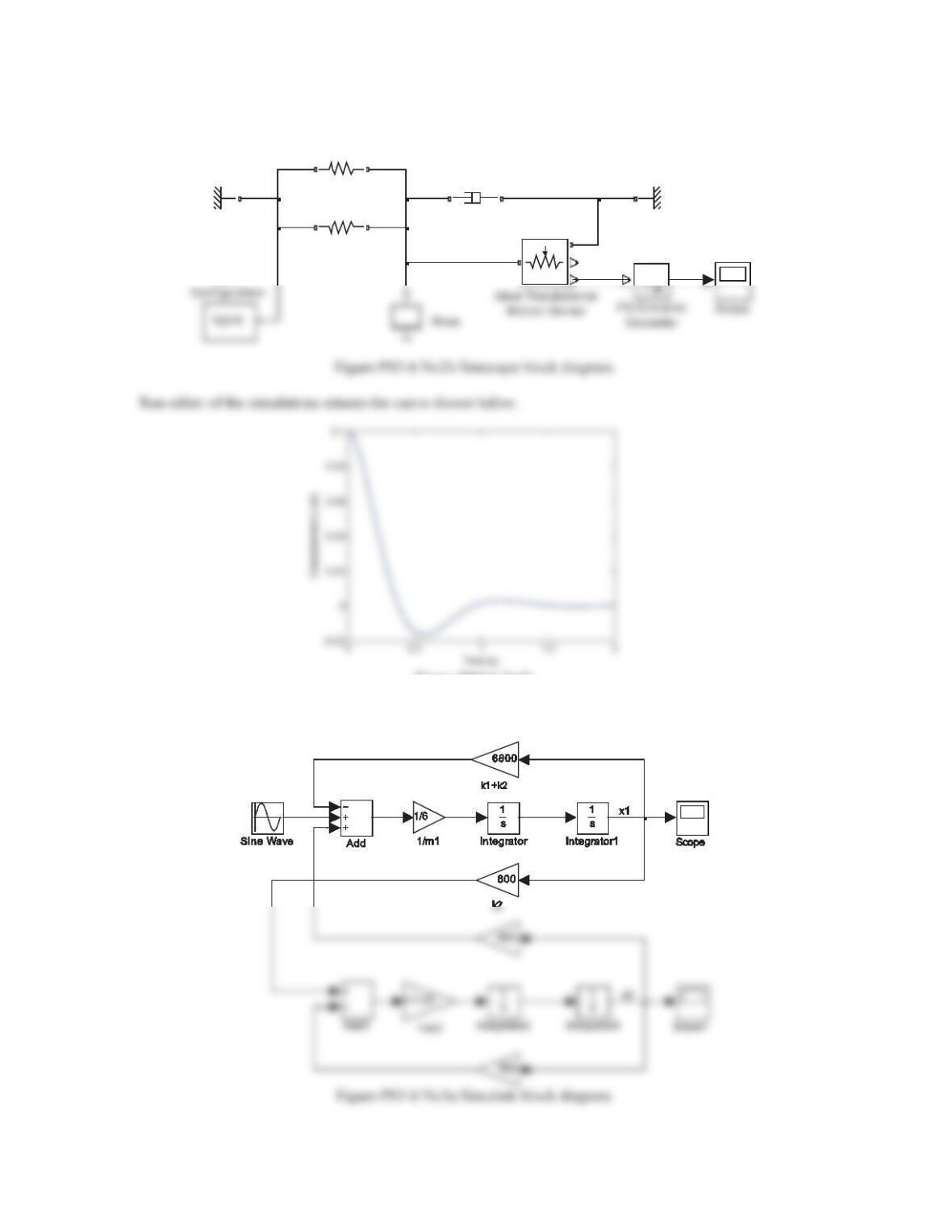
a. Build a Simulink model based on the differential equations of motion of the system and find the
displacement outputs x1(t) and x2(t).
b. Build a Simscape model of the physical system and find the displacement outputs x1(t) and x2(t).
Solution
The differential equations of motion of the system is
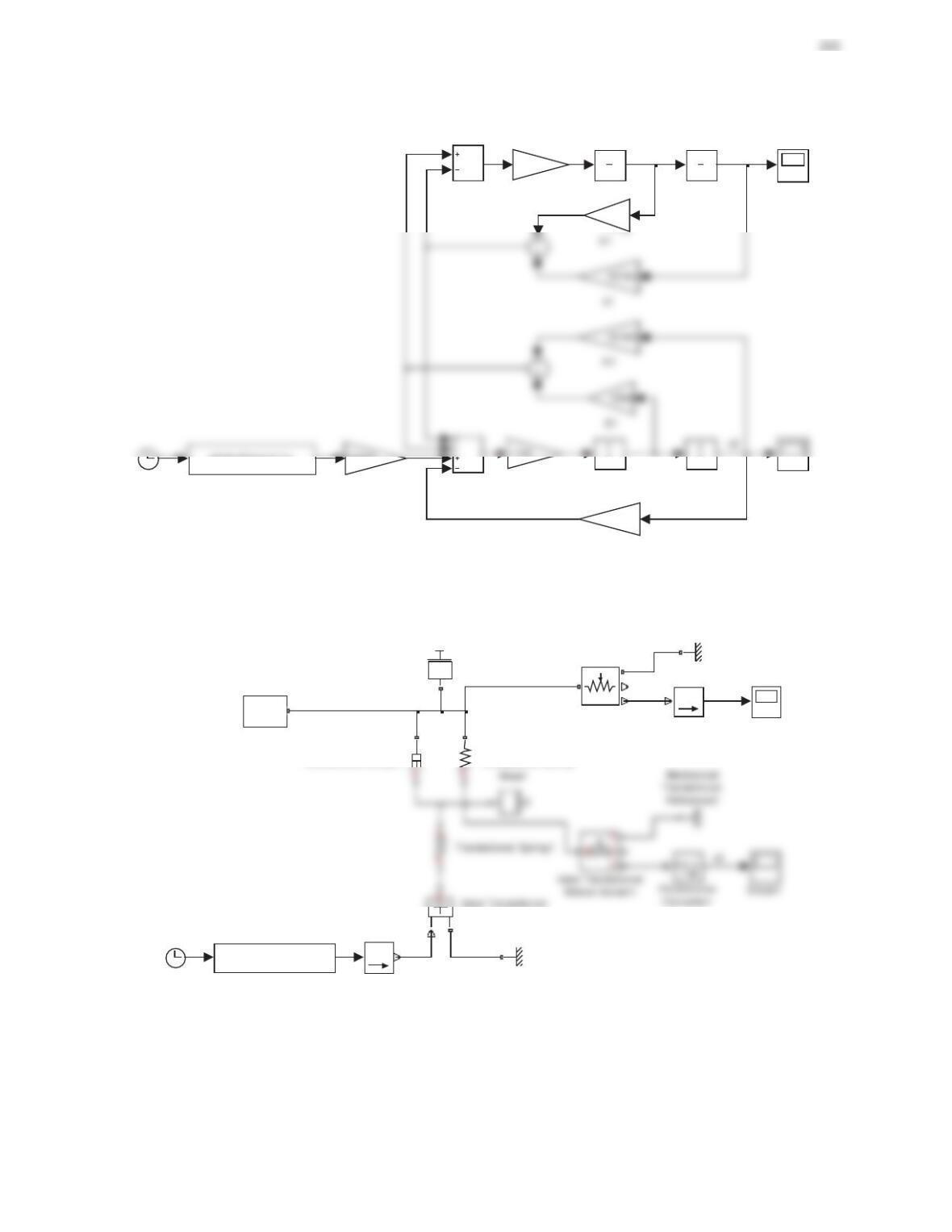
4. Repeat Problem 3 for the two-degree-of-freedom quarter-car model in Example 5.5. Assume that the
surface of the road can be approximated as a sine wave z=Z0sin(Svt/L), where Z0= 0.01, L= 10m, and the
speed v= 20 km/h. If the car moves at a speed of 100 km/h, rerun the simulations and compare the results with
those obtained in the case of 20 km/h. Ignore the control force ffor both cases.
Solution
The differential equations of motion of the system is
5. Consider the disk-shaft system in Problem 2 of Problem Set 5.3. The system is approximated as a single-
degree-of-freedom rotational mass–spring system, where m= 10 kg, r= 0.05 m, and K= 1000 Nm/rad.
a. Assume that a torque W=50u(t) Nm is acting on the disk, which is initially at rest. Build a Simscape model
of the physical system and find the angular displacement output T(t).
b. Assuming that the external torque is W= 0 and the initial angular displacement is T(0) = 0.1 rad, find the
angular displacement output T(t).
Solution
199
2
1
2
șș IJmr K
6. Consider the pendulum-bob system in Problem 5 of Problem Set 5.3. The parameter values are m= 0.1 kg,
M= 1.2 kg, L= 0.6 m, and B= 0.5 Ns/m. The initial angular displacement is T(0) = 0.1 rad and the initial
angular velocity is
ș UDGV
.
a. Build a Simulink block diagram based on the nonlinear mathematical model of the system and find the
angular displacement output T(t).
b. Build a Simscape model of the nonlinear physical system and find the angular displacement output T(t).
Solution
The nonlinear mathematical model of the system is
2
11
32
sin 0mML B mMgLTT T
MATLAB Figures
Problem 1
200
Run either of the simulations returns the curve shown below.
Problem 2
Figure PS5-6 No2a Simulink block diagram.
0
2
4
8
10
12
14 x 10-3
Displacement x (m)
201
Figure PS5-6 No2c
Problem 3
CR
Translational
Damper
CR
Translational
Spring1
CR
Translational
Spring
Solver
SPS
Mechanical
Translational
Reference1
Mechanical
Translational
Reference
P
V
C
R
202
Figure PS5-6 No3b Simscape block diagram.
Run either of the simulations returns the curves shown below.
x2
Translational
f(x)=0
Solver
Configuration
Scope1
SPS
PS-Simulink
Converter1
Mechanical
M a ss1
P
V
C
R
Ideal Translational
Motion Sensor1
-0.1
0.1
0.15
-0.1
0.1
0.15
Problem 4
Figure PS5-6 No4a Simulink block diagram.
Figure PS5-6 No4b Simscape block diagram.
x1
19000
k2
1000
Scope1
Scope
19000
K2
s
Integrator3
s
Integrator2
1
s
Integrator1
1
s
Integrator
z0*sin(2*pi*v/L*u)
Fcn
Clock
Add1
Add
1/m2
1/290
1/m1
x1
CR
Translational Spring
CR
Translational Damper
f(x)=0
Solver
Configuration
SPS
Simulink-PS
Converter1
Scope
SPS
PS-Simulink
Converter
Mechanical
Translational
Reference1
Mechanical
Translational
Reference
Mass
C
S
Velocity Source
P
V
C
R
Ideal Translational
Motion Sensor
z0*2*pi*v/L*cos(2*pi*v/L*u)
Fcn
velocity z_dot
Clock
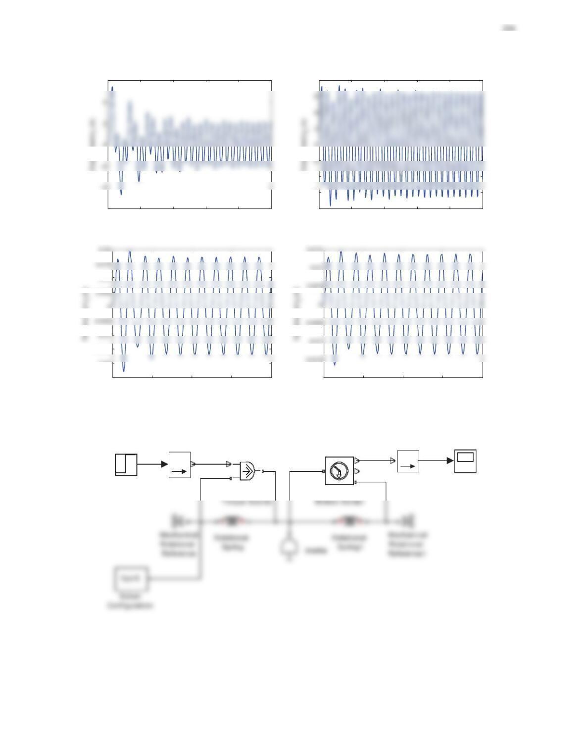
Figure PS5-6 No4c: v= 100 km/h
Figure PS5-6 No4c: v= 20 km/h
Problem 5
Figure PS5-6 No5a Simscape block diagram.
0 2 46810
-6
6x 10
-3
Time (s)
0 2 4 6 8 10
-8
-6
-4
8x 10
-3
Time (s)
0 5 10 15 20
-0.025
-0.02
-0.015
0.01
Time (s)
0 5 10 15 20
-0.02
Time (s)
theta
Step
SPS
Simulink-PS
Converter
Scope
SPS
PS-Simulink
Converter
A
W
C
R
Ideal Rotational
R
C
S
Ideal
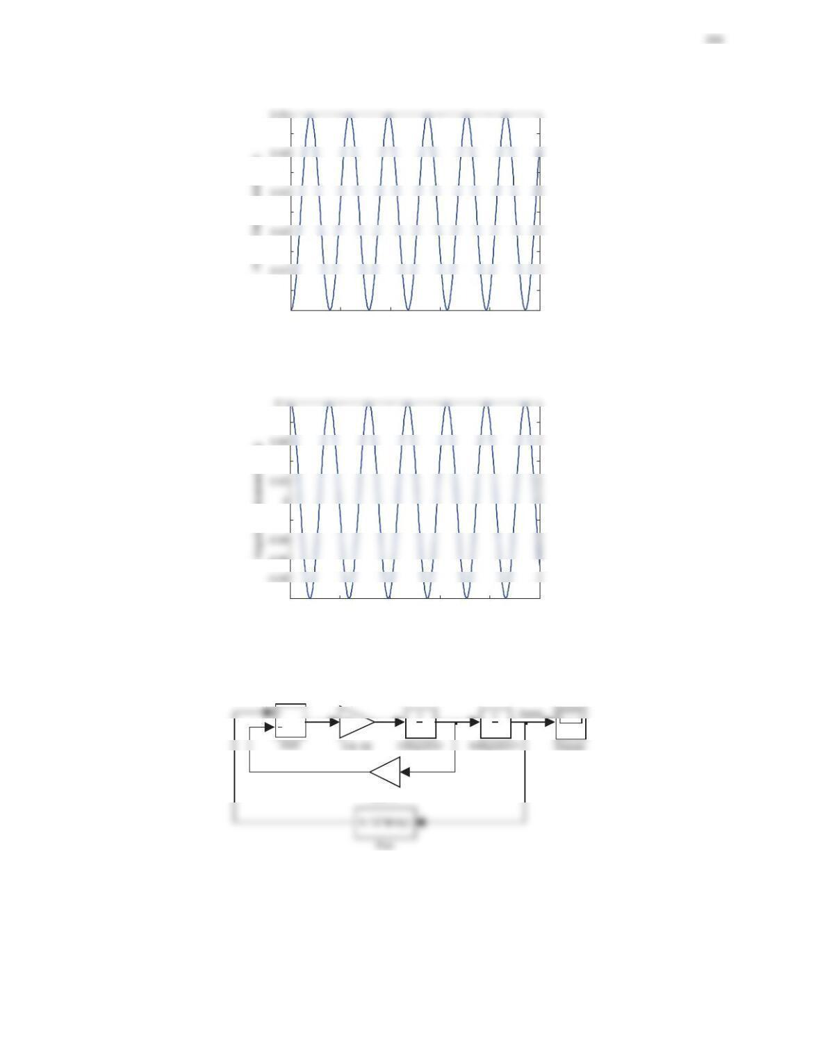
Figure PS5-6 No5b Angular displacement output.
Set the external torque Was 0 and the initial angular displacement T(0) as 0.1 rad.
Figure PS5-6 No5c Angular displacement output.
Problem 6
Figure PS5-6 No6a Simulink block diagram.
Rewrite the equation as
0.18 0.5 4.12sinT T T
,where
4.12sinT
is considered as a torque applied to the
system.
00.02 0.04 0.06 0.08 0.1
0
0.005
0.015
0.025
0.035
0.045
Time (s)
T (rad)
00.02 0.04 0.06 0.08 0.1
-0.1
-0.06
-0.02
0.04
0.08
Time (s)
T (rad)
s
s
0.5
Gain1
-K-
206
Figure PS5-6 No6b Simscape block diagram.
Run either of the simulations returns the curve shown below.
Figure PS5-6 No6c
Review Problems
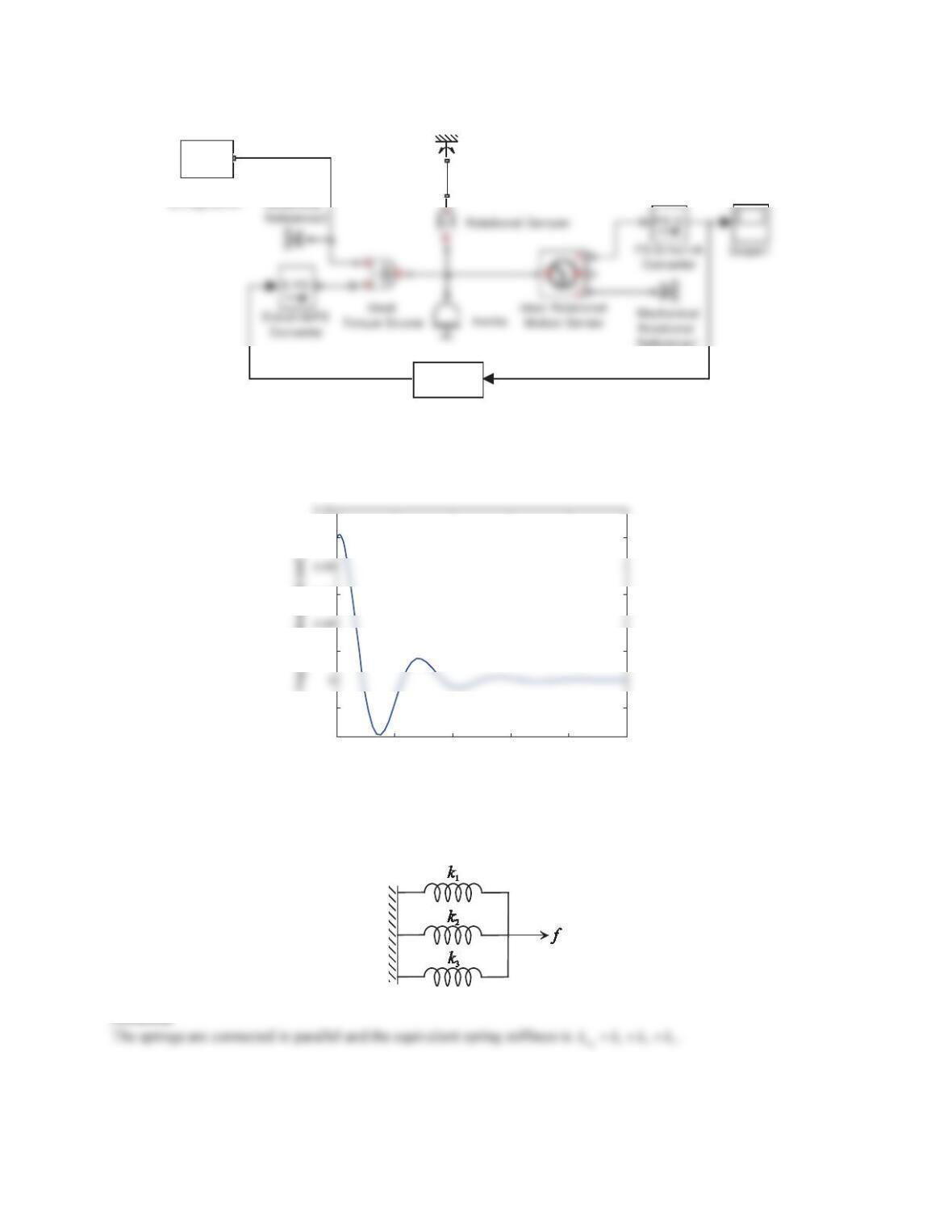
1. Determine the equivalent spring constant for the system shown in Figure 5.119.
Figure 5.119 Problem 1.
Solution
2. Determine the equivalent spring constant for the system shown in Figure 5.120.
f(x)=0
Solver
Configuration
Mechanical
Reference1
Mechanical
Rotational
Reference
-4.12*sin(u)
Fcn
0 1 2 3 4 5
-0.04
-0.02
0.02
0.06
0.1
Time (s)
207
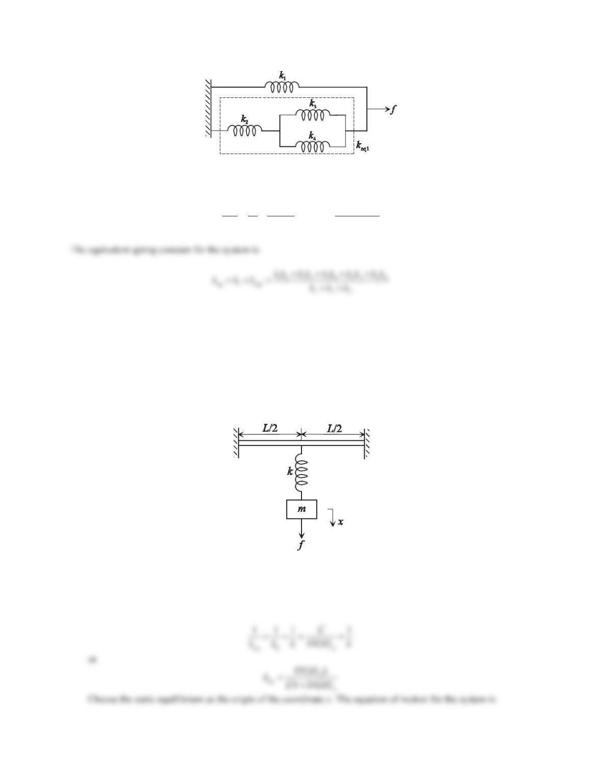
Figure 5.120 Problem 2.
Solution
The equivalent spring constant for the bottom part is
eq1 2 3 4
11 1
kkkk
or
23 24
eq1
234
kk kk
kkkk
3. Consider the system shown in Figure 5.121, where a mass–spring system is hung from the middle of a massless
beam. Assume that the beam can be modeled as a spring and the equivalent stiffness at the midspan is
192EIA/L3, where Eis the modulus of elasticity of beam material and IAis the area moment of inertia about the
beam’s longitudinal axis.
a. Derive the differential equation of motion for the system.
b. Using the differential equation obtained in Part (a), determine the transfer function X(s)/F(s). Assume that
the initial conditions are x(0) = 0 and
(0) 0x
.
c. Using the differential equation obtained in Part (a), determine the state-space representation. Assume that
the output is the displacement xof the mass.
Figure 5.121 Problem 3.
Solution
a. The system is equivalent to the mass-spring system shown in the figure below, where the spring kbrepresents
the flexibility of the beam and kb= 192EIA/L3. The equivalent spring stiffness of the system is


