419
Problem Set 10.1
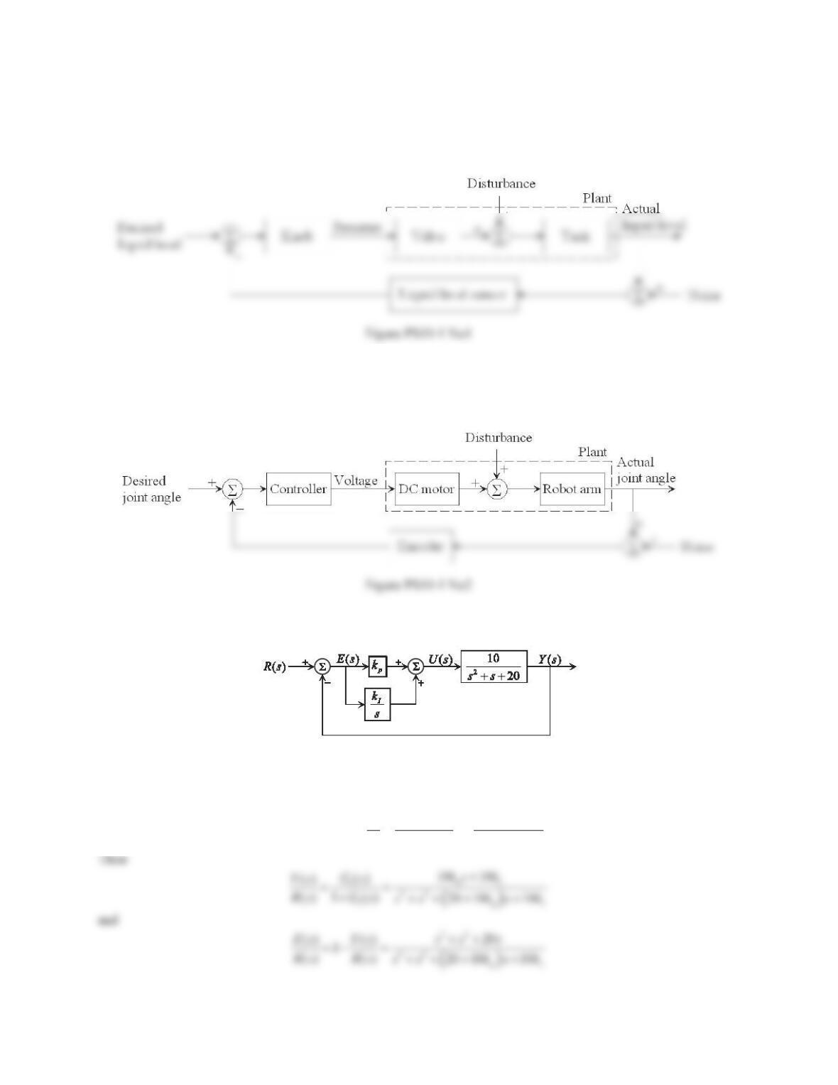
1. Draw a block diagram for the feedback control of a liquid-level system, which consists of a valve with a control
knob (0–100%) and a liquid-level sensor. Clearly label essential components and signals.
Solution
2. Draw a block diagram for the feedback control of a single-link robot arm system, which consists of a DC motor
to produce the driving force and an encoder to measure the joint angle. Clearly label essential components and
signals.
Solution
3. Determine the transfer functions U(s)/E(s), Y(s)/R(s), and E(s)/R(s) in Figure 10.4.
Figure 10.4 Problem 3.
Solution
By block algebra, the equivalent transfer function for the forward path is
pI
I
1p 232
10 10
10
() 20 20
ks k
k
Gs k sss ss s
§·
§·
¨¸
¨¸
©¹
©¹
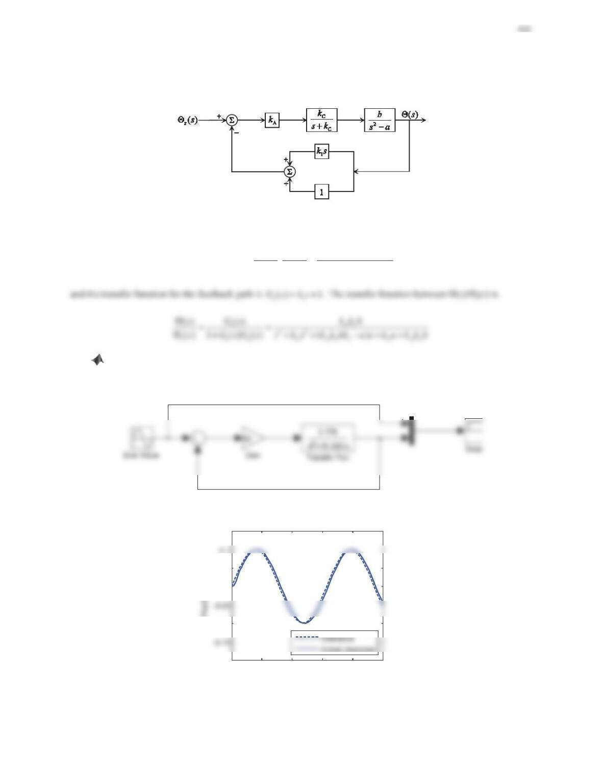
4. The block diagram in Figure 10.5 represents a rocket attitude control system. Determine the transfer function
4(s)/4r(s).
Figure 10.5 Problem 4.
Solution
By block algebra, the transfer function for the forward path is
CAC
1A 232
CCC
() kkkb
b
Gs k sk s a s ks aska
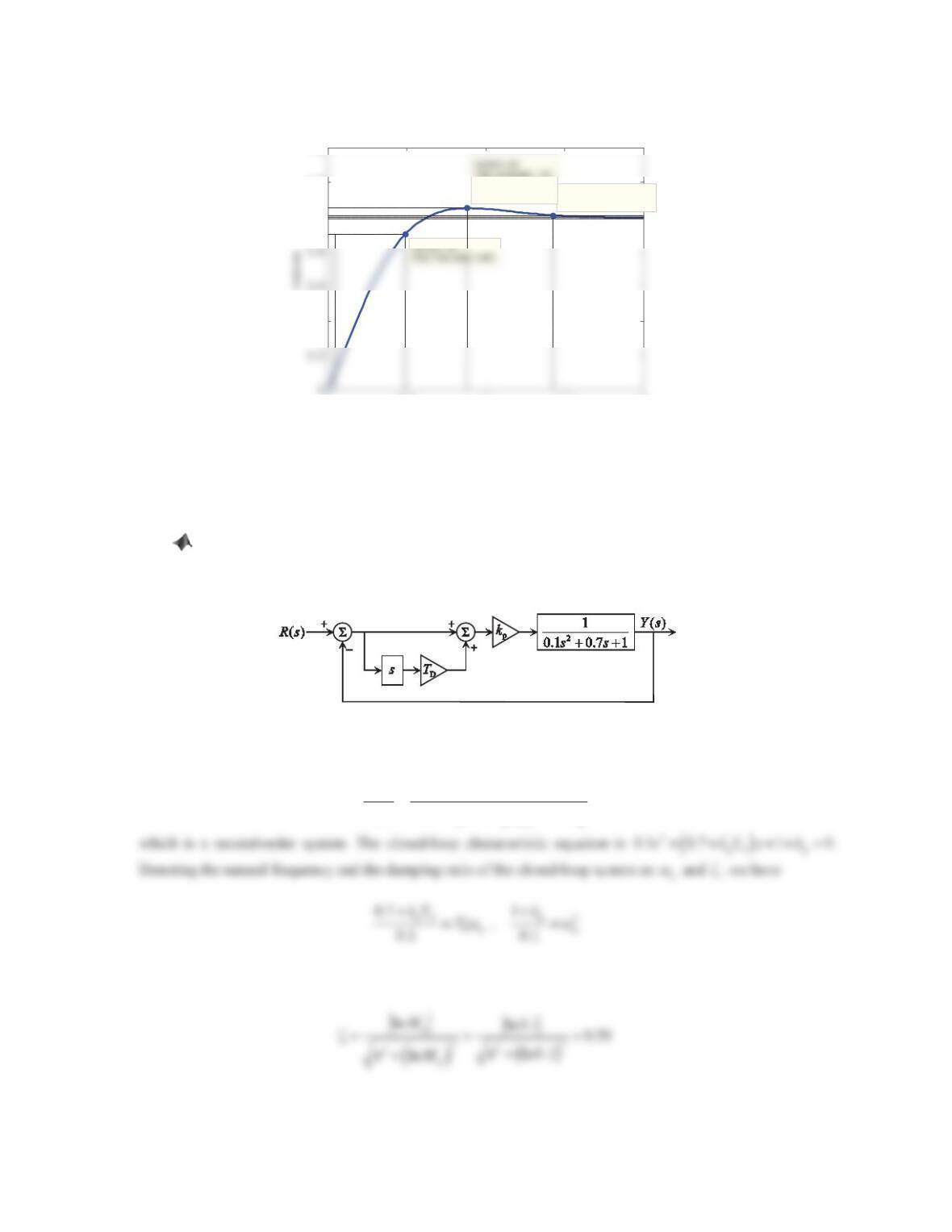
5. Consider the control system in Example 10.2. Build a Simulink block diagram to simulate reference
tracking control, where the signal R(s) is a sine wave with a magnitude of 0.1 m and a frequency of 2 rad/s. Show
the actual position response and the reference signal in the same scope.
Solution
Figure PS10-1 No5a Simulink block diagram.
0 1 2 3 4 5
-0.2
-0.1
0
0.05
0.15
Time (s )
Figure PS10-1 No5b Responses.
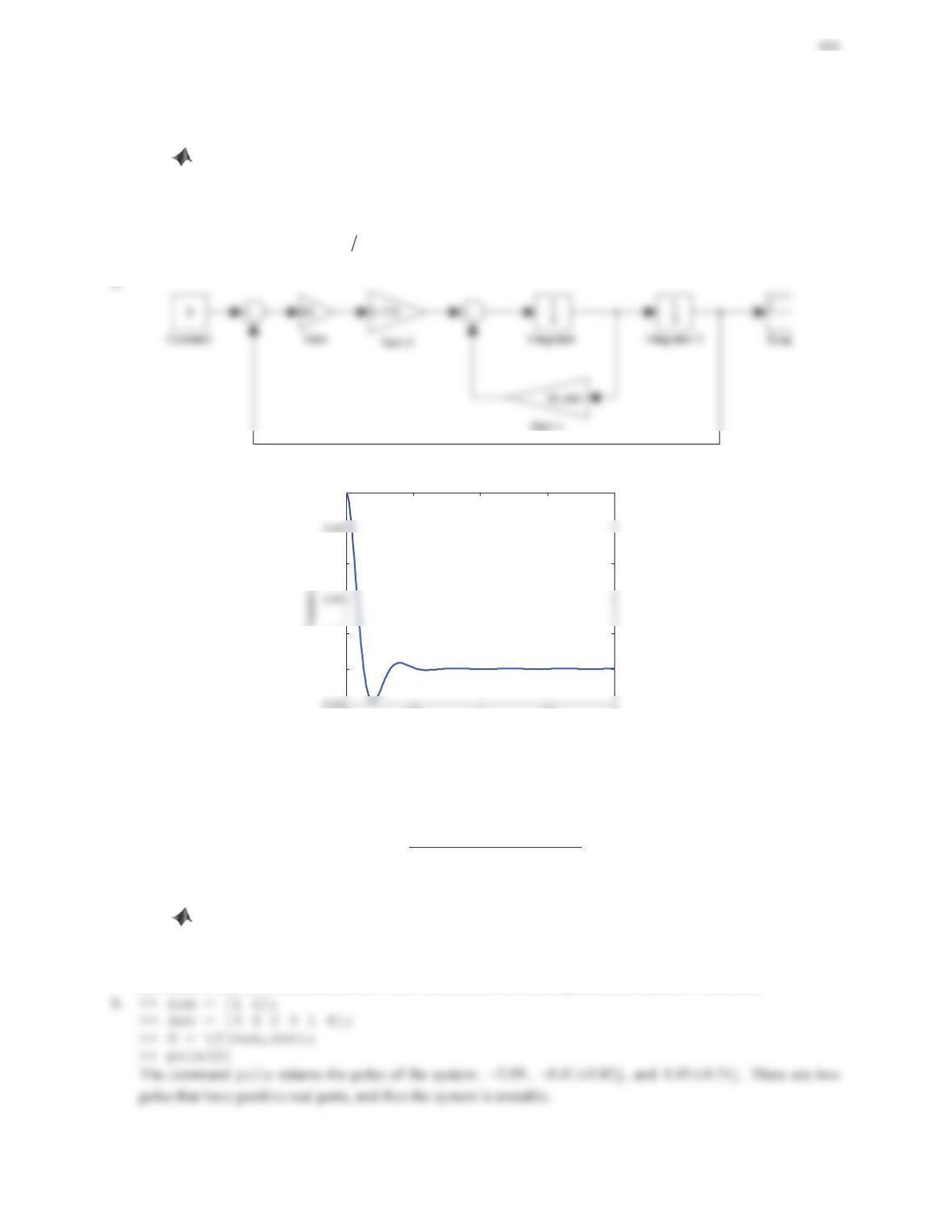
6. Reconsider the control system in Example 10.2.
a. Convert the transfer function G(s) = Y(s)/U(s) to a differential equation of y(t).
b. Using the differential equation obtained in Part (a) to represent the plant, build a Simulink block
diagram to simulate regulation control, where the reference signal R(s) is zero. Assume that the initial
conditions are y(0) = 0.1 m and (0) 0y
m/s.
Solution
a. The transfer function () () ()Gs Y s U s in Example 10.2 can be written as
( ) 16.883 ( ) 3.778 ( )yt yt ut
.
Figure PS10-1 No6a Simulink block diagram.
00.5 11.5 2
0
0.02
0.06
0.1
Time (s)
Figure PS10-1 No6b Responses.
Problem Set 10.2
1. The transfer function of a dynamic system is given by
5432
1
() .
3625 4
s
Gs sssss
a. Using Routh’s stability criterion, determine the stability of the system.
b. Using MATLAB, solve for the poles of the system and verify the result obtained in Part (a).
Solution
a. The characteristic equation of the closed-loop system is 5432
3625 4sssss
. The Routh array can be
formed as follows. Since the elements in the first column are not all positive, the system is unstable.
422
5
4
:3 21
:6 54
s
s
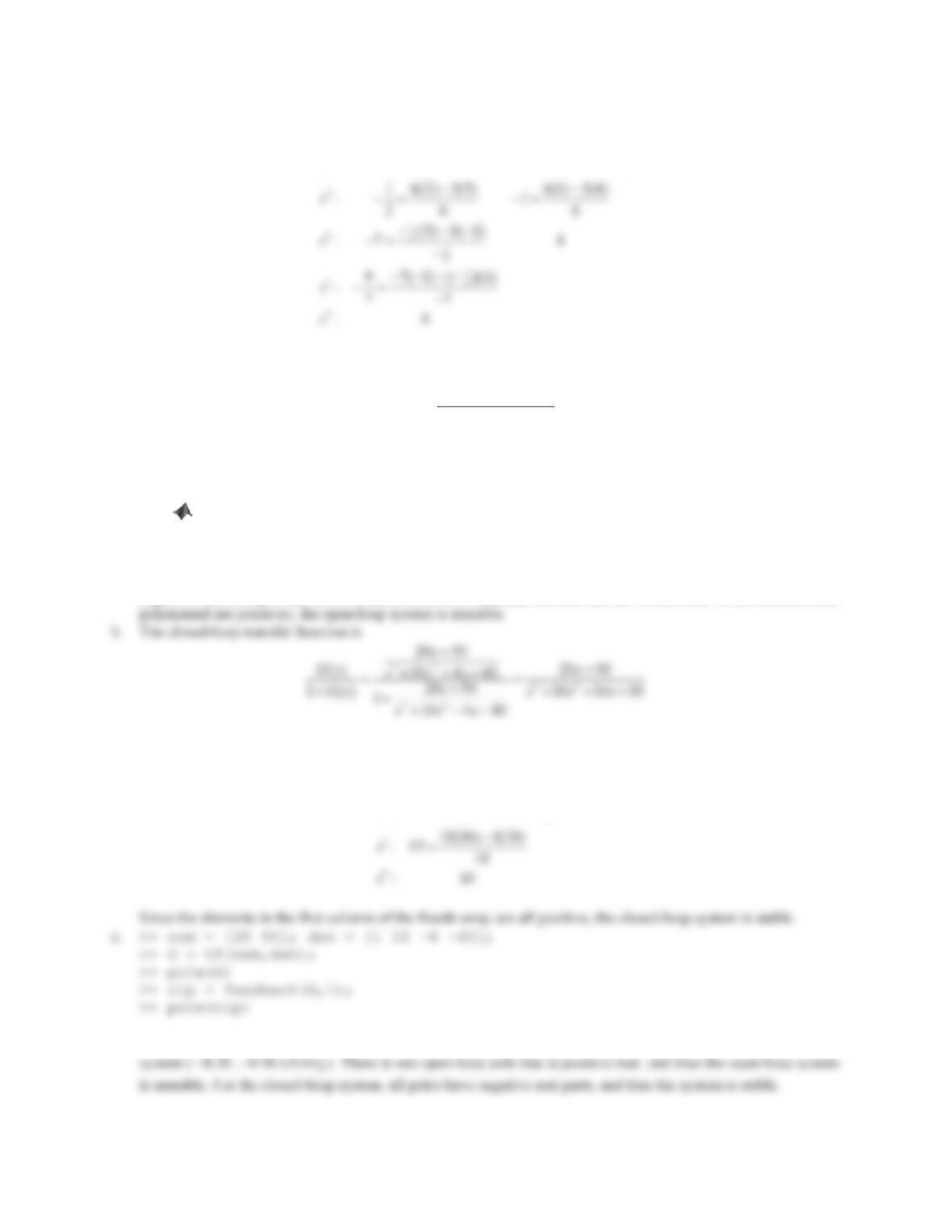
2. The transfer function of a dynamic system is given by
32
20 50
() .
10 440
s
Gs sss
a. Using Routh’s stability criterion, determine the stability of the open-loop system.
b. Suppose that a negative unity feedback is applied to this open-loop system. Using Routh’s stability
criterion, determine the stability of the resulting closed-loop system.
c. Using MATLAB, solve for the poles of the open-loop and closed-loop systems and verify the results
obtained in Parts (a) and (b).
Solution
a. For the open-loop system, the characteristic equation is
32
10 40 04sss
, where two coefficients are
negative. According to the first condition of Routh’s stability criterion (all the coefficients of the characteristic
Thus, the characteristic equation of the closed-loop system is
32
1601010sss
. The Routh array can be
formed as follows.
3
2
:116
:1010
s
s
The command pole returns the poles of the open-loop system (
10
,
2
, 2) and those of the closed-loop
423
3. The unit-step response for a second-order system
22 2
nnn
// 2Ys Us s s Z ]Z Z
is given by
ndd
2
() 1 e cos sin .
1
t
yt t t
]Z ]
ªº
«»
«»
¬
Z Z
]¼
Prove that the relationship between the overshoot Mpand the damping ratio is
2
/1
p
e.M
S] ]
Solution
Differentiating
()yt
with respect to t, we obtain
nn
ȗȦ ȗȦ
nd d dd dd
22
ȗȗ
() ȗȦ FRV Ȧ VLQ Ȧ Ȧ VLQ Ȧ Ȧ FRVȦ
1ȗȗ
tt
yt e t t e t t
§·§ ·
¨¸¨ ¸
¨¸¨ ¸
©¹© ¹
Note that the time derivative
()yt
equals zero when
()yt
reaches its maximum value at the peak time
p
t
,
This occurs when
dp
sin Ȧt
. Therefore, we have
The overshoot
p
M
can be determined by computing
p
()1yt
,which is
2
ʌȗ ȗ
p
Me
.
4. Consider a second-order system
22 2
nnn
// 2Ys Us s s Z ]Z Z
, which has two poles at 3±4j.
a. Determine the undamped natural frequency Zn, damping ratio ], and damped natural frequency Zdof the
system.
b. Estimate the rise time tr, overshoot Mp, peak time tp, and 2% settling time tsin the unit-step response for the
system.
Solution
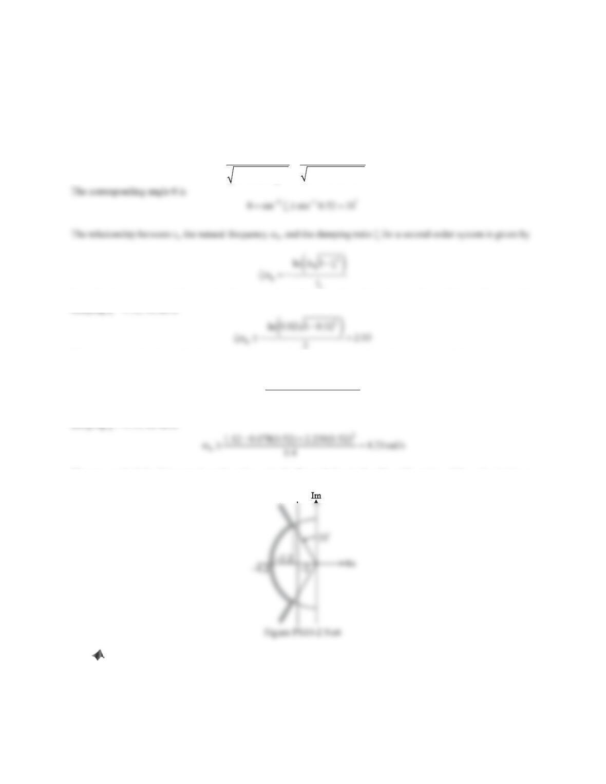
a. For a second-order system with two poles at 3±4j, the undamped natural frequency Zn, damping ratio ], and
damped natural frequency Zdare

424
b. The rise time trcan be solved from the equation
The overshoot Mpand peak time tpare
p9.e48e%MS] ] S ,p
d
49tSS
Zs
The 2% settling time tsis
5. Consider a second-order system
22 2
nnn
// 2Ys Us s s Z ]Z Z . Sketch the allowable region of the
poles in the s-plane if the requirements for the system’s unit-step response are Mp% and rise time tr
s.
Solution
For Mp10 %, we have
The approximated relationship between tr,WKH QDWXUDO IUHTXHQF\ Ȧn, and the damping ratio ]for a second-order
system is given by
r
The natural frequency Ȧnincreases with increasing damping ratio ] For time tr s and the smallest possible
damping ȗ= 0.59, we have
The area to the left of the gray boundary shown in the figure below is the allowable region for the poles in the s–
plane so that the two performance requirements are met.
425
6. Consider a second-order system
22 2
nnn
// 2Ys Us s s Z ]Z Z . Sketch the allowable region of the
poles in the s–plane if the requirements for the system’s unit-step response are Mp15%, 2% settling time ts
s, and rise time tr s.
Solution
For Mp15 %, we have
p
222 2
p
|ln | | ln 0.15 | 0.52
(ln ) (ln 0.15)
M
M
] t
S S
Note that ȗZnincreases with increasing damping ratio ȗ. Thus, for 2% settling time ts s and the smallest possible
damping ȗ= 0.52, we have
The approximated relationship between tr,WKH QDWXUDO IUHTXHQF\ Ȧn, and the damping ratio ]for a second-order
system is given by
2
n
r
1.12 0.078 2.230
t
]]
Z|
The natural frequency Ȧnincreases with increasing damping ratio ] For time tr s and the smallest possible
damping ȗ= 0.52, we have
The area to the left of the gray boundary shown in the figure below is the allowable region of the poles in the
s
–
plane so that the two performance requirements are met.
7. Consider a second-order system
22 2
nnn
// 2Ys Us s s Z ]Z Z
. Write a MATLAB m–file to plot
WKHPDJQLWXGHRIWKHV\VWHP¶VIUHTXHQF\UHVSRQVHIXQFWLRQIRUWKHIROORZLQJFDVHVȦn UDGVDQGȗ
0.1, 0.5, and 1. Summarize the effects of the damping ratio on the frequency-domain performance.
426
Solution
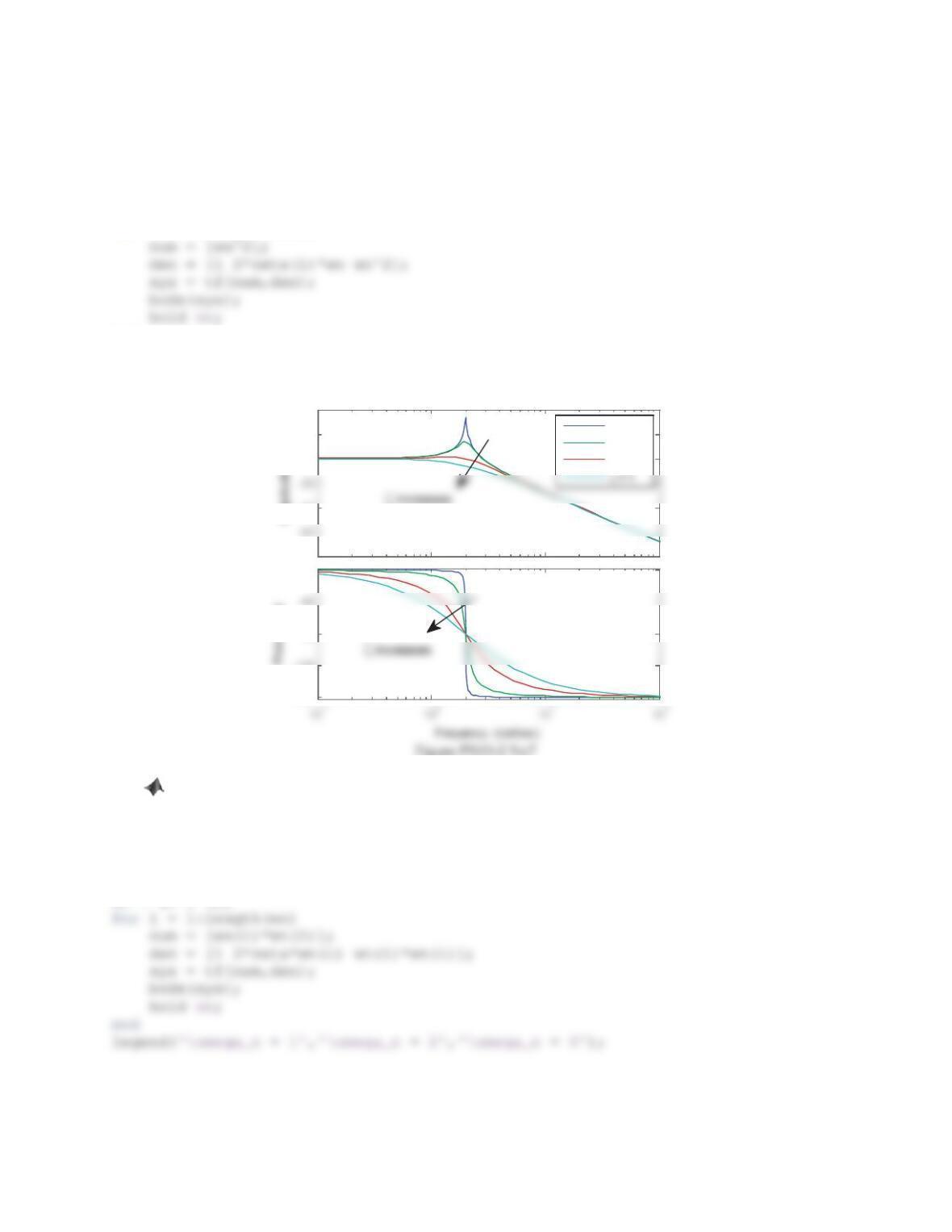
As shown in the figure below, the resonant peak is related to the damping of the system. The smaller the damping,
the higher the resonant peak.
wn = 2;
zeta = [0.01 0.1 0.5 1];
for i = 1:length(zeta)
end
legend(‘\zeta = 0.01’,‘\zeta = 0.1’,‘\zeta = 0.5’,‘\zeta = 1’);
-80
-40
0
20
40
Magnitude (dB)
–180
–135
-90
0
Bode Diagram
] = 0.01
] = 0.1
] = 0.5
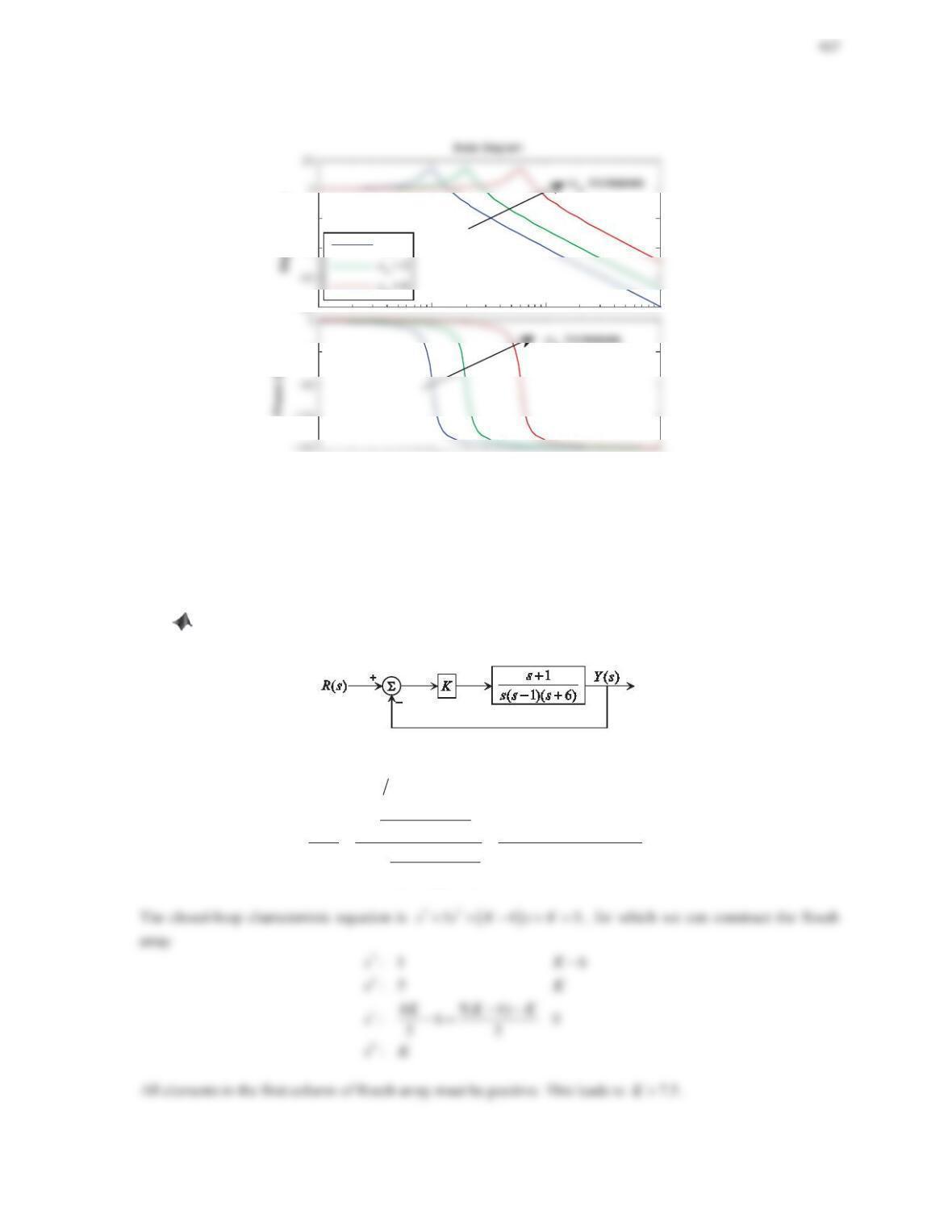
8. Repeat Problem 7 for the following caVHVȗ DQGȦn= 1, 2, and 6 rad/s. Summarize the effects of the
natural frequency on the frequency-domain performance.
Solution
As shown in the figure below, the bandwidth is related to the natural frequency of the system. The bandwidth
increases when the natural frequency increases.
zeta = 0.1;
wn = [1 2 6];
-80
-40
-20
10
-1
10
0
10
1
10
2
–135
-45
Frequency (rad/sec)
Z
n
= 1
n
Figure PS10-2 No8
Problem Set 10.3
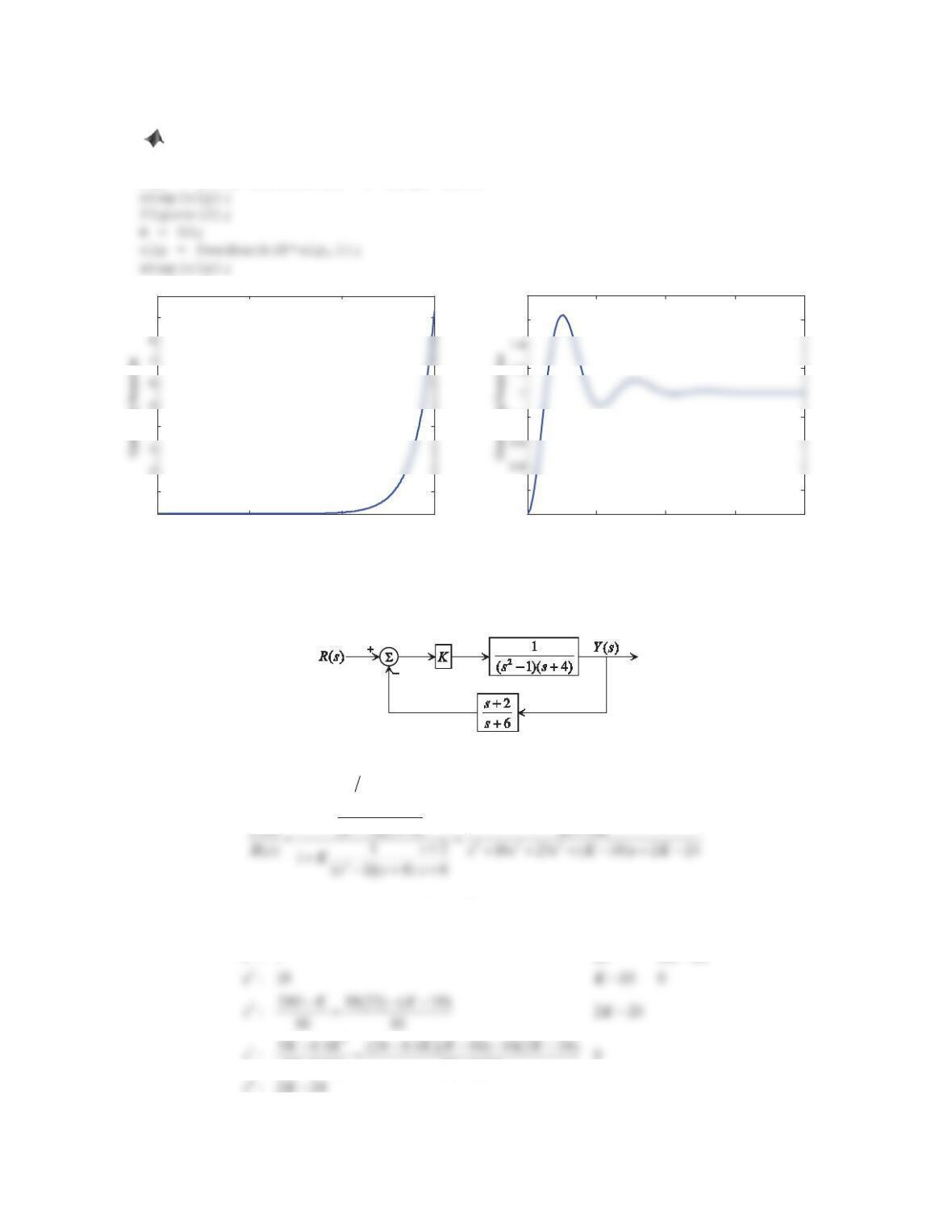
1. Consider the feedback system shown in Figure 10.24.
a. Using Routh’s stability criterion, determine the range of the control gain Kfor which the closed-loop
system is stable.
b. Use MATLAB commands to find the unit-step responses for open-loop and closed-loop control.
Assume that the control gain is K= 50. Compare the open- and closed-loop responses.
Figure 10.24 Problem 1.
Solution
a. The closed-loop transfer function () ()Ys Rs is
32
1
16
()
1
() 5 6
116
s
Kss s
Ys Ks K
s
Rs s s K s K
Kss s
428
b. Below is the MATLAB session.
figure(1);
olp = tf([1 1],conv([1 -1 0],[1 6]));
0 5 10 15
0
1
4
9
10 x 105
Time (s)
0 1 2 3 4
0
0.2
0.8
1.2
1.6
1.8
Time (s)
Figure PS10-3 No1
2. Consider the feedback system shown in Figure 10.25. Using Routh’s stability criterion, determine the range of
the control gain Kfor which the closed-loop system is stable.
Figure 10.25 Problem 2.
Solution
The closed-loop transfer function () ()Ys Rs is
2
1
() 6
K
Ys Ks K
The closed-loop characteristic equation is
432
10 23 ( 10) 2 24 0sssKsK
, for which we can construct the
Routh array
4
: 1 23 2 24
24 0.1 24 0.1
sK
sKK
sK
429
In order to make the closed-loop system stable, all elements in the first column of Routh array must be positive,
24 0.1 0 240
KK
!o
3. Reconsider Example 10.6. Using the final value theorem, verify the steady-state errors to a unit-step input for
open-loop and closed-loop control without and with disturbance.
Solution
For the open-loop system, we have
where
2.5K
. The steady-state value of
()yt
is
ss 00 0 0
41 10
lim ( ) lim ( ) ( ) lim 2.5 lim 1
10 10
ss s s
ysYssKGsRss
ss s
oo o o
(without disturbance)
where
2.5K
. The steady-state value of
()yt
is
ss 00 0 0
50 4
( ) 1 200
lim ( ) lim ( ) lim lim 0.95
1 ( ) 10 4 50 210
ss s s
KG s
ysYss Rss
KG s s s s
oo o o
(without disturbance)
4. A stable system can be classified as a system type, which is defined as the degree of the polynomial for which
the steady-state error is a nonzero finite constant. For instance, if the error to a step input, which is a polynomial
of zero degree, is a nonzero finite constant, then such a system is called type 0, and so on. Consider the system
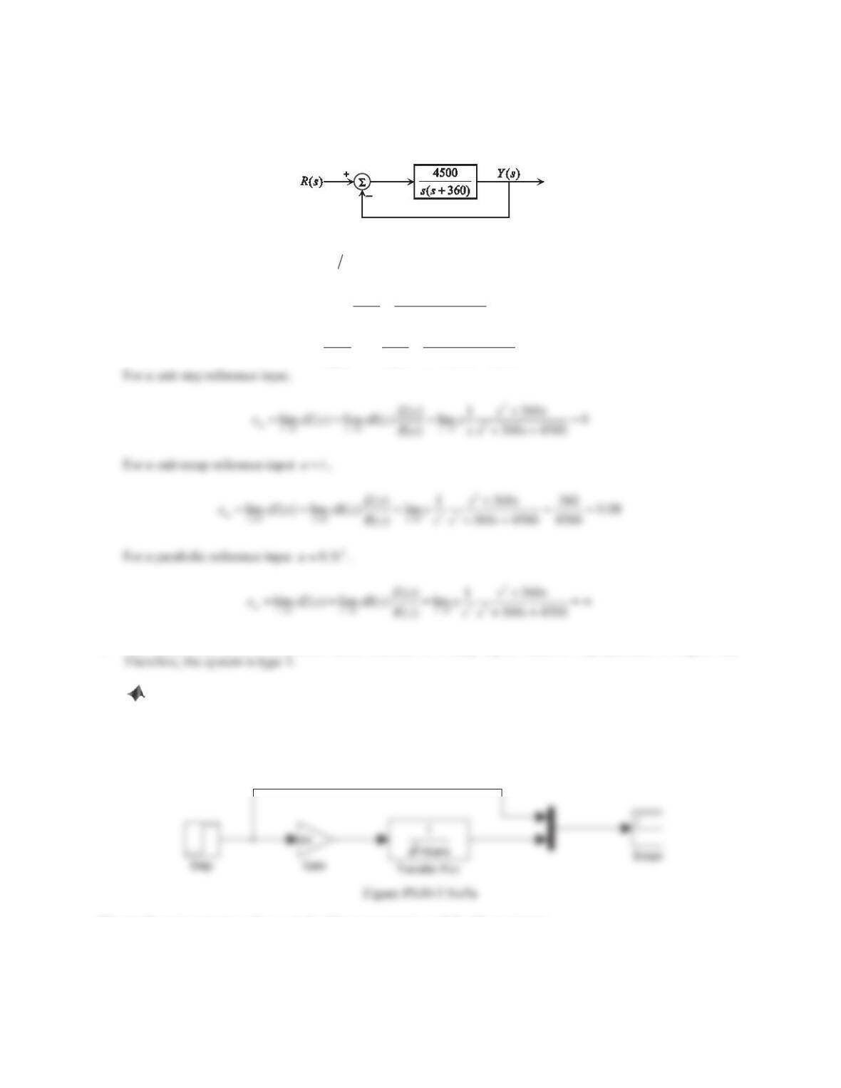
in Figure 10.26.
430
a. Compute the following steady-state errors: (1) for a unit-step reference input, (2) for a unit-ramp reference
input u=t, and (3) for a parabolic reference input u= 0.5t2.
b. Determine the system type.
Figure 10.26 Problem 4.
Solution
a. The closed-loop transfer function () ()Ys Rs is
2
( ) 4500
( ) 360 4500
Ys
Rs s s
2
2
() () 360
1
( ) ( ) 360 4500
Es Ys s s
Rs Rs s s
b. The steady-state error is a nonzero finite constant to a ramp input, which is a polynomial of degree one.
5. Reconsider Example 10.8. Build Simulink block diagrams to simulate open-loop and closed-loop control
with parameter variations. Verify the steady-state response values yss obtained in Example 10.8.
Solution
The Simulink block diagram for open-loop control is shown below, where k= 40 without uncertainty or 50 with
uncertainty.
The steady-state response value yss is 1 without uncertainty or 0.8 with uncertainty.
0 2 4 6 8 10
0
0.2
0.6
1
1.2
Time (s)
No uncertainty
With uncertainty
Figure PS10-3 No5b
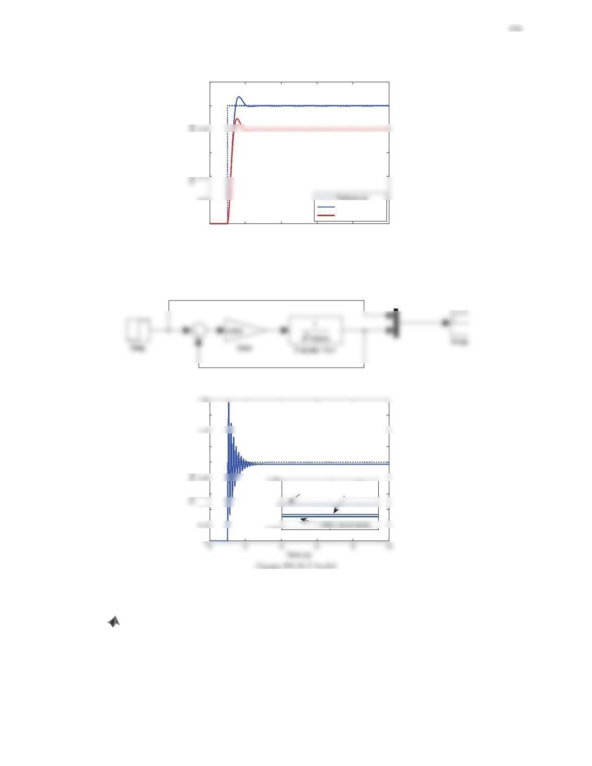
The Simulink block diagram for closed-loop control is shown below. The steady-state response value yss is
about 0.98 without uncertainty or 0.97 with uncertainty.
Figure PS10-3 No5c
0.4
1
1.2
1.6
99.5 10
0.95
1.05
Reference No
Uncertainty
6. Consider the feedback control system shown in Figure 10.27.
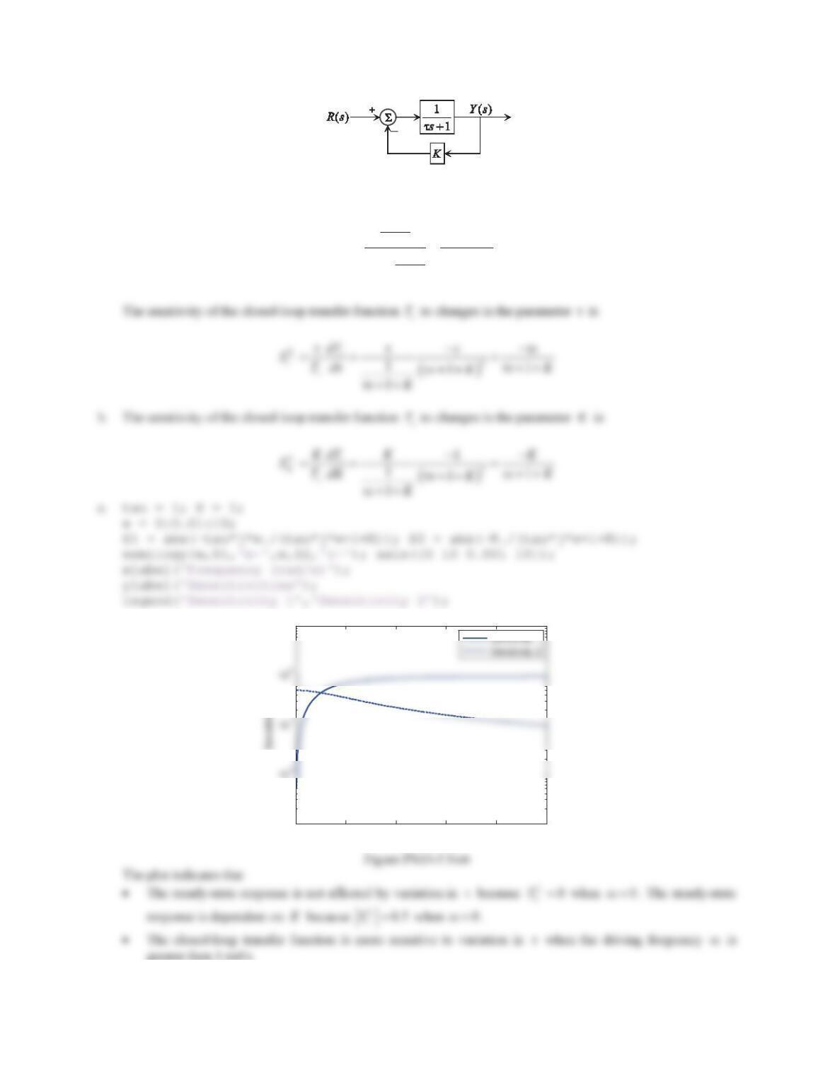
a. Compute the sensitivity of the closed-ORRSWUDQVIHUIXQFWLRQWRFKDQJHVLQWKHSDUDPHWHUIJ.
b. Compute the sensitivity of the closed-loop transfer function to changes in the parameter K.
c. $VVXPLQJIJ DQGK= 1, use MATLAB to plot the magnitude of each of the sensitivity functions for
s MȦ8VHWKHORJDULWKPLFVFDOHIRUWKHy–D[LV&RPPHQWRQWKHHIIHFWRISDUDPHWHUYDULDWLRQVLQIJDQGK
IRUGLIIHUHQWGULYLQJIUHTXHQFLHVȦ.
432
Figure 10.27 Problem 6.
Solution
a. The closed-loop transfer function is
1
1
IJ
1IJ
1IJ
c
s
TsK
Ks
0 2 4 6 8 10
10
-3
10
1
Frequency (rad/s)
433
Problem Set 10.4
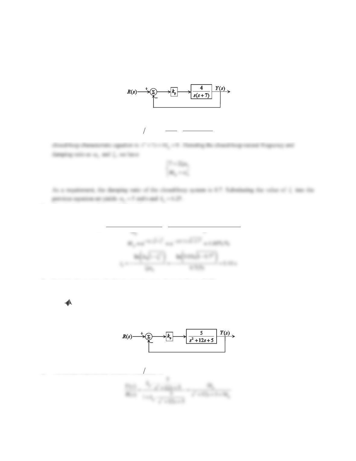
1. Figure 10.38 shows a negative feedback control system.
a. Design a P controller such that the damping ratio of the closed-loop system is 0.7.
b. Estimate the rise time, overshoot, and 1% settling time in the unit-step response for the closed-loop system.
Figure 10.38 Problem 1.
Solution
a. The closed-loop transfer function () ()Ys Rs is
p
2
p
4
()
() 7 4
k
Ys
Rs s s k
, which is a second-order system. The
b. The rise time, overshoot, and 1% settling time are
22
r
1.12 0.078 2.230 1.12 0.078(0.7) 2.230(0.7) 0.43
t]]
|
s
2. Consider the negative feedback control system shown in Figure 10.39.
a. Design a P controller such that the maximum overshoot in the response to a unit-step reference input is less
than 15%, the 2% settling time is less than 1 s, and the rise time is less than 0.2 s.
b. Use MATLAB to plot the unit-step response of the closed-loop system. Find the overshoot, 2%
settling time, and rise time. If the time-domain specifications exceed the requirements, make a fine tuning
and reduce them to be approximately the specified values or less.
Figure 10.39 Problem 2.
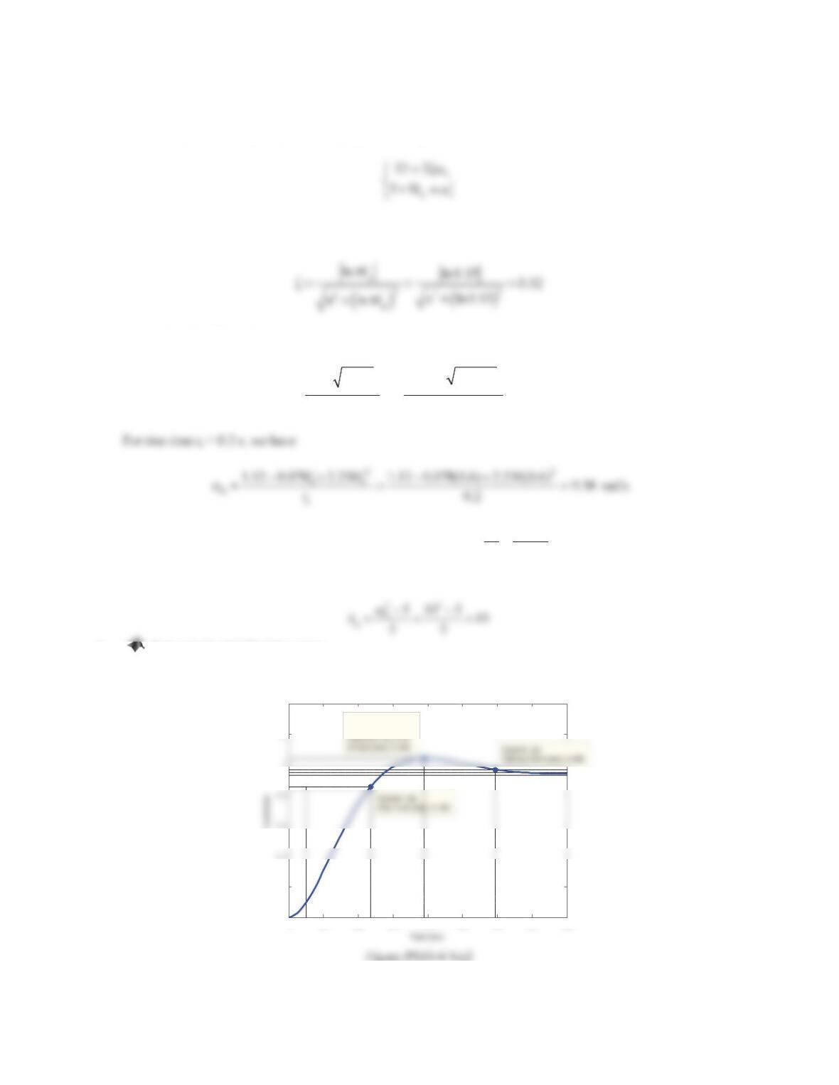
Solution
a. The closed-loop transfer function () ()Ys Rs is
434
which is a second-order system. The closed-loop characteristic equation is
2
p
12 5 5 0ss k
. Denoting the
closed-loop natural frequency and damping ratio as
n
Ȧ
and
ȗ
, we have
The requirement of overshoot
p
15%M
implies that
Let ȗ= 0.6. For 2% settling time ts< 1 s, we have
22
n
s
ln 1 ln 0.02 1 0.6
6.89
0.6t
‘]
Z !
]
rad/s
Also, from the closed-loop characteristic equation, we have
n
12 12
Ȧ
2ȗ
rad/s. In order to satisfy all
three conditions, pick n
Ȧ rad/s. Thus, the control gain can be determined as
b. Below is the MATLAB session.
sys = tf([5],[1 12 5]); kp = 19; clp = feedback(kp*sys,1); step(clp);
S t ep Res ponse
00.1 0.2 0.3 0.4 0.5 0.6 0.7 0.8
0
0.2
1.2
1.4
System: clp
Peak amplitude: 1.04
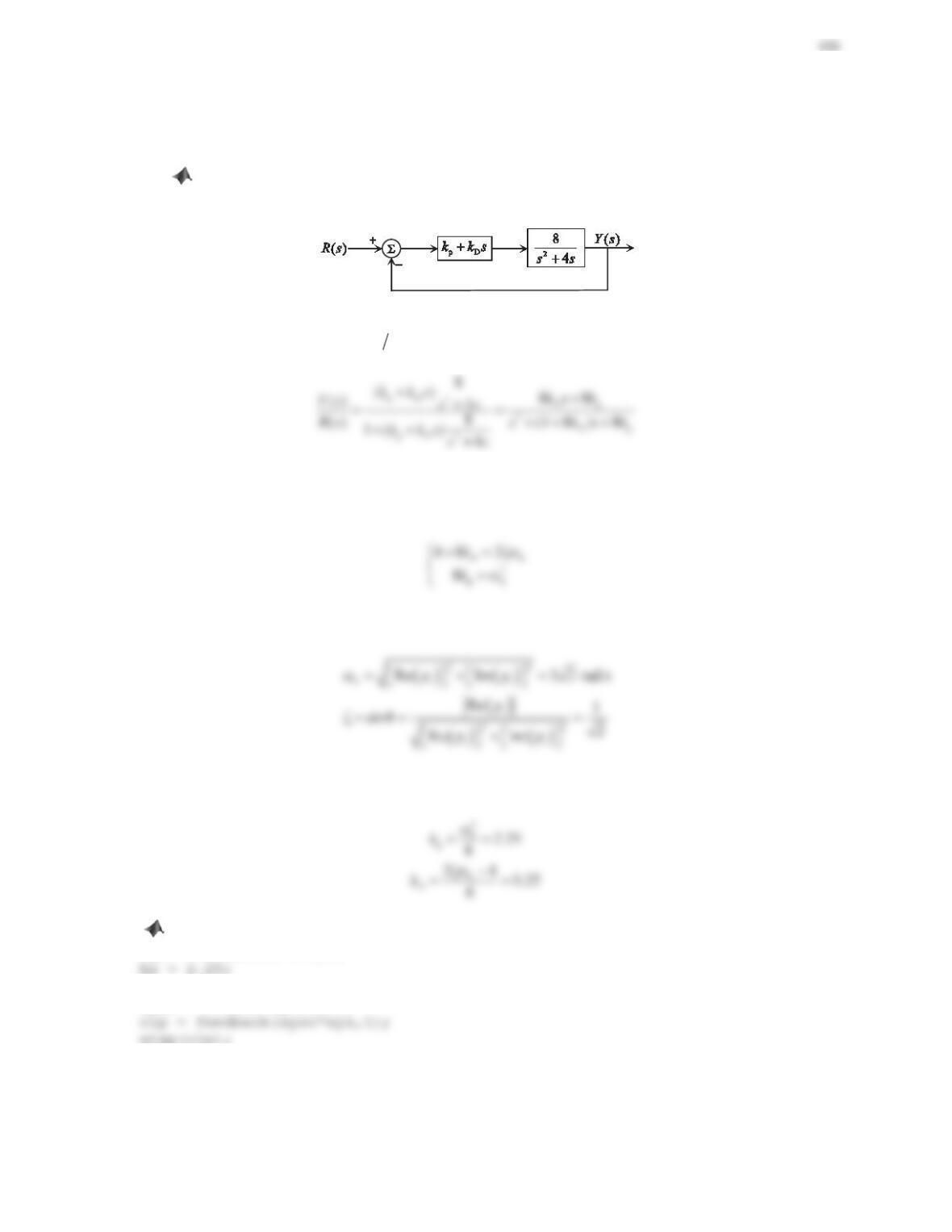
3. Consider the feedback control system shown in Figure 10.40.
a. Design a PD controller such that the closed-loop poles are at p1,2 =3±3j.
b. Use MATLAB to plot the unit-step response of the closed-loop system. Find the rise time, overshoot,
peak time, and 1% settling time.
Figure 10.40 Problem 3.
Solution
a. The closed-loop transfer function () ()Ys Rs is
which is a second-order system. The closed-loop characteristic equation is
2
Dp
(4 8 ) 8 0sksk
.Denoting
the closed-loop natural frequency and damping ratio as
n
Ȧ
and
ȗ
, we have
As a requirement, the closed-loop poles are located at
1,2
33jp r
. This implies that
where 1i or 2. Substituting the values of
n
Ȧ
and
ȗ
into the previous equation set yields
b. Below is the MATLAB session.
sys = tf([8],[1 4 0]);
kd = 0.25;
sysc = tf([kd kp],[1]);
436
S t ep Res ponse
Time (sec)
00.5 11.5 2
0.4
1
1.2
1.4
System: clp
Settling Time (sec): 1.43
Overshoot (%): 5.12
At time (sec): 0.883
Figure PS10-4 No3
4. Consider the feedback control system shown in Figure 10.41.
a. Find the values for kpand TDsuch that the maximum overshoot in the response to a unit-step reference
input is less than 10% and the 1% settling time is less than 0.5 s.
b. Compute the steady-state error of the closed-loop system to a unit-step reference input.
c. Verify the results in Parts (a) and (b) using MATLAB by plotting the unit-step response of the closed-
loop system. If the maximum overshoot and the settling time exceed the requirements, make a fine tuning
and reduce them to be approximately the specified values or less.
Figure 10.41 Problem 4.
Solution
a. The closed-loop transfer function
pD p
2
pD p
()
() 0.1 0.7 1
kT s k
Ys
Rs skTsk
The requirement of overshoot p
10%M
implies that
n
s
0.75(0.5)t
]
Choosing
0.75
]
and
n
Ȧ
yields
p
21.5k
and
D
0.07T
.
b. For a unit step reference input,
c. Below is the MATLAB session.
sys = tf([1],[0.1 0.7 1]); kp = 21.5; Td = 0.07;
sysc = tf([kp*Td kp],[1]); clp = feedback(sysc*sys,1);
step(clp);
Step Response
Amplitude
00.1 0.2 0.3 0.4 0.5 0.6 0.7
0
0.2
0.6
0.8
1.2
1.4
System: clp
Peak amplitude: 1.05
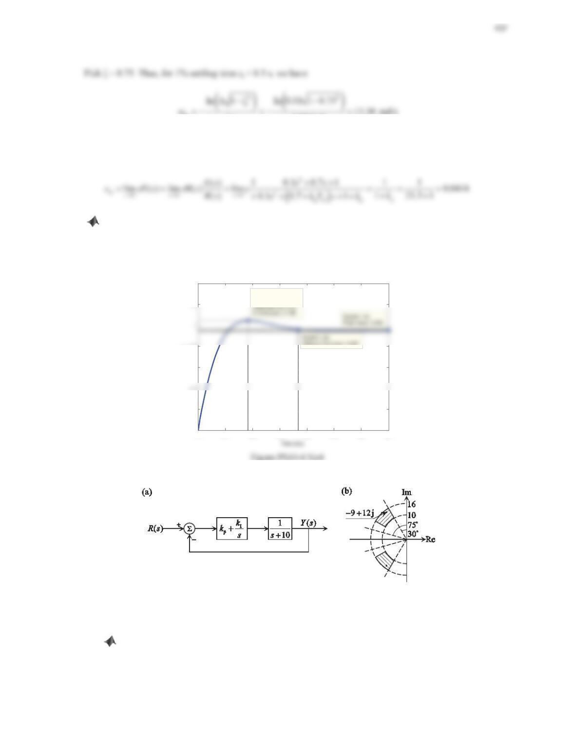
5. Consider the feedback control system shown in Figure 10.42a.
Figure 10.42 Problem 5.
a. If the desired closed-loop poles are located within the shaded regions shown in Figure 10.42b, determine
the corresponding rangeVRIȦnDQGȗRIWKHFORVHG-loop system.
b. Design a PI controller such that the closed-loop poles are at p1,2 =í9±12j.
c. Compute the steady-state errors of the plant and the closed-loop system to a unit-step reference input.
d. Verify the results in Part (c) using MATLAB by plotting the unit–step responses of the plant and the
closed-loop system.
438
Solution
a. Note that the semicircles in Figure 10.42(b) indicate lines of constant natural frequencies
n
Ȧ
and the diagonal
lines indicate constant damping ratios
ȗ
. Thus, for the shaded regions, we have
10 rad/s Ȧ UDGVdd
b. The closed-loop transfer function () ()Ys Rs is
which is a second-order system. The closed-loop characteristic equation is
2
pI
(10 ) 0sksk
. Denoting the
natural frequency and the damping ratio of the closed-loop system as
n
Ȧ
and
ȗ
, we have
As a requirement, the closed-loop poles are located at
1,2 912pj r
. This implies that
where 1i , 2. Substituting the values of
n
Ȧ
and
ȗ
into the previous equation set yields I225k and p8k .
c. The steady-state value of the unit step response of the plant is
d. Below is the MATLAB session.
sys = tf([1],[1 10]);