134
Problem Set 5.1
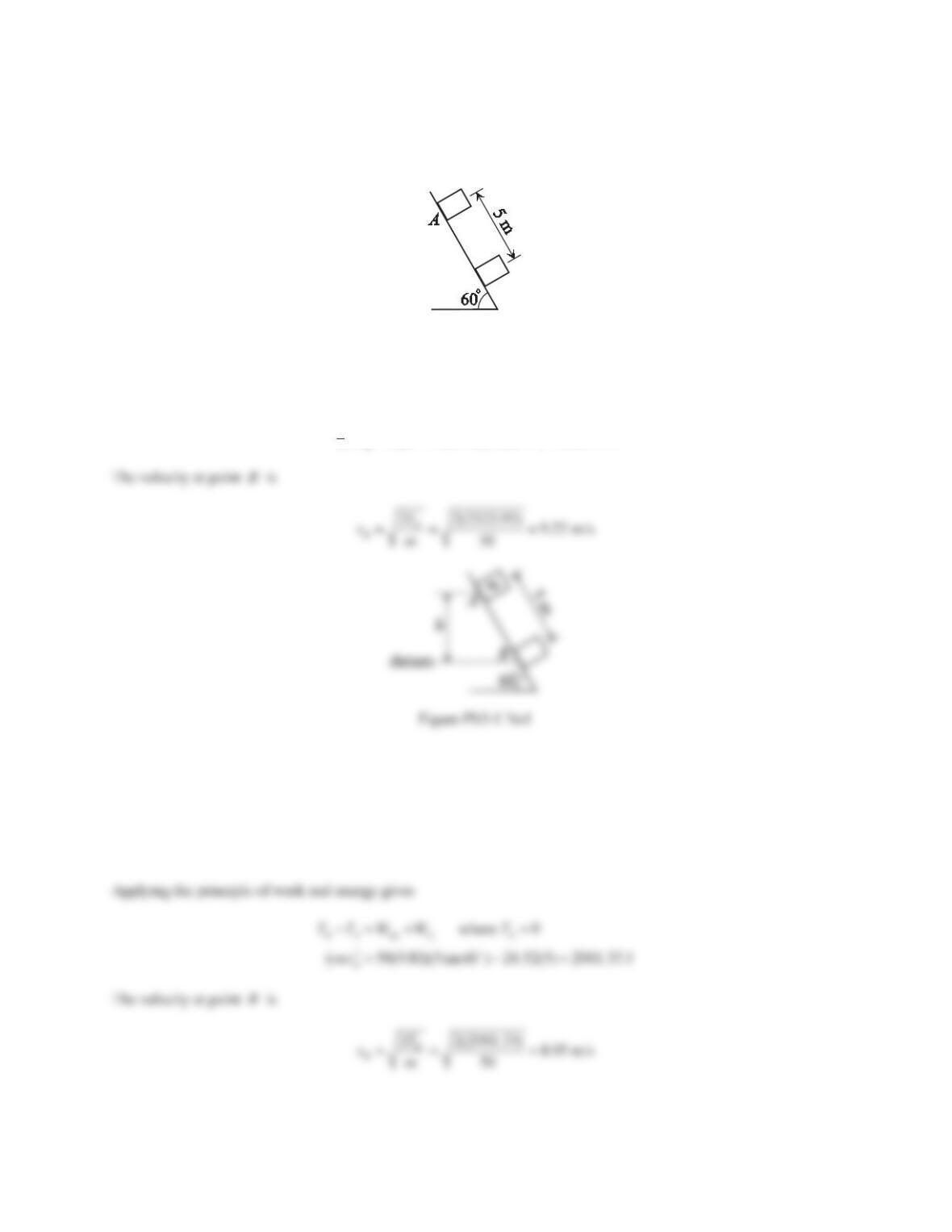
1. If the 50–kg block in Figure 5.12 is released from rest at A, determine its kinetic energy and velocity after it
slides 5 m down the plane. Assume that the plane is smooth.
Figure 5.12 Problem 1.
Solution
Choosing point Bas the datum and applying the principle of conservation of energy gives
2
1
2
where 0 and 0
50(9.81)(5sin 60 ) 2123.93 J
BB AA B A
B
TV TV V T
mv mgh
D
2. 5HSHDW3UREOHPLIWKHFRHIILFLHQWRINLQHWLFIULFWLRQEHWZHHQWKHEORFNDQGWKHSODQHLVȝk= 0.1.
Solution
From the free-body diagram shown below, we obtain the friction force
ȝ ȝ FRV FRV 1
fk k
FNmg
DD
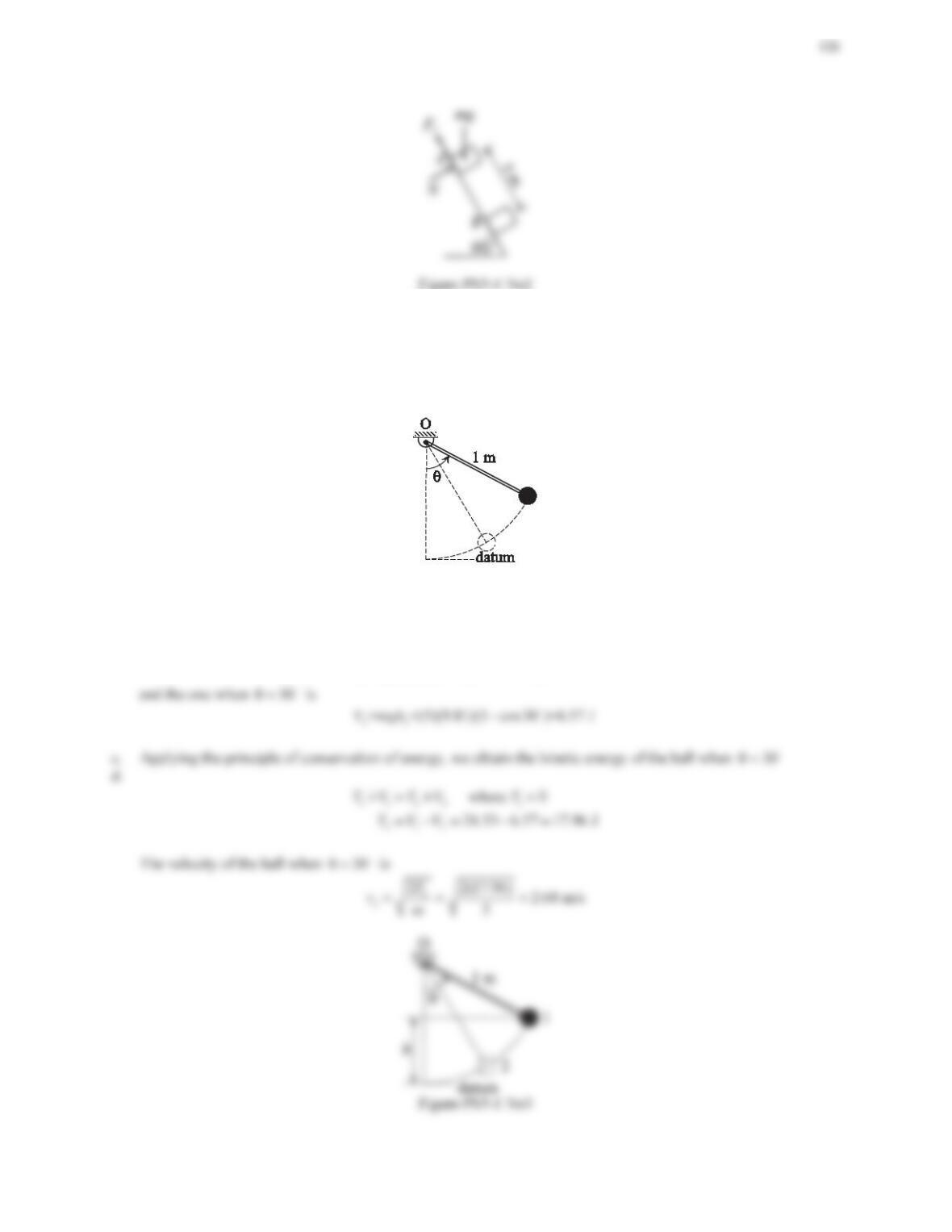
3. The ball in Figure 5.13 has a mass of 5 kg and is fixed to a rod having a negligible mass. Assume that the ball is
UHOHDVHGIURPUHVWZKHQș 60°.
a. Determine the gravitational potentiDOHQHUJ\RIWKHEDOOZKHQș 0° and 30°. The datum is shown in
Figure 5.13.
b. Determine the kinetic energ\DQGWKHYHORFLW\RIWKHEDOOZKHQș °.
Figure 5.13 Problem 3.
Solution
a. With the chosen datum, the gravitational potential energy of the ball when
ș D
is
b.
11
= =(5)(9.81)(1 cos60 )=24.53 JVmgh D
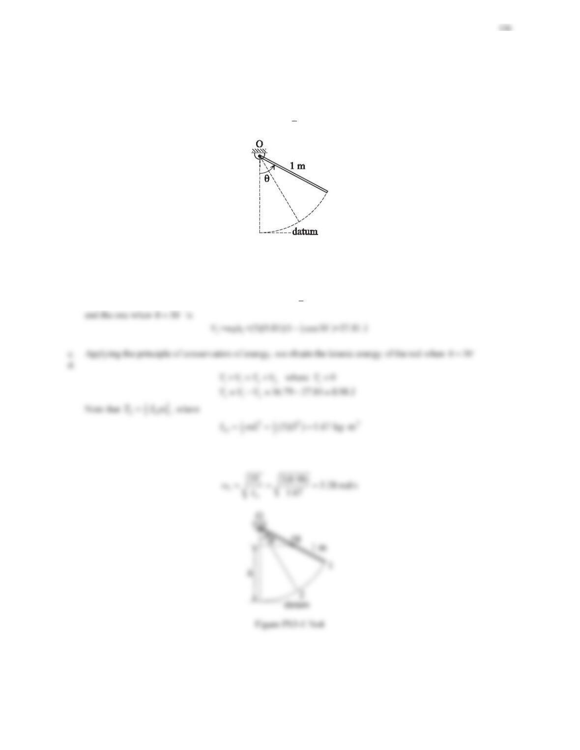
4. The 5-NJVOHQGHUURGLQ)LJXUHLVUHOHDVHGIURPUHVWZKHQș 60°.
a. ‘HWHUPLQH WKH JUDYLWDWLRQDO SRWHQWLDO HQHUJ\ RI WKH URG ZKHQ ș 60° and 30°. The datum is shown in
Figure 5.14.
b. Determine the NLQHWLFHQHUJ\DQGWKHDQJXODUYHORFLW\RIWKHURGZKHQș °. The mass moment of inertia
of the slender rod about the fixed point O is
2
1
O3
ImL
,where Lis the length of the rod.
Figure 5.14 Problem 4.
Solution
a. With the chosen datum, the gravitational potential energy of the rod when
ș D
is
b.
1
11 2
= =(5)(9.81)(1 cos60 )=36.79 JVmgh D
The angular velocity of the rod when
ș
D
is
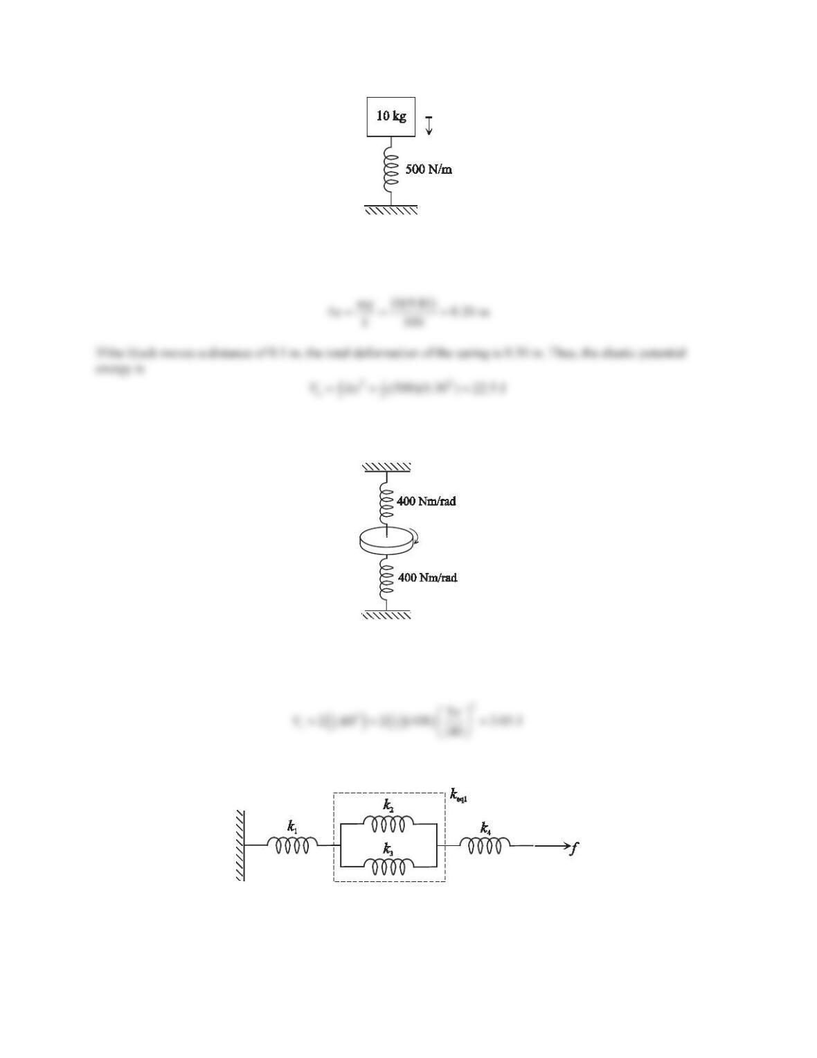
5. Determine the elastic potential energy of the system shown in Figure 5.15 if the 10-kg block moves downward a
distance of 0.1 m. Assume that the block is originally in static equilibrium.
137
Figure 5.15 Problem 5.
Solution
Since the block is originally in static equilibrium, the spring is compressed and the deformation is
6. If the disk in Figure 5.16 rotates in the clockwise direction by 5°, determine the elastic potential energy of the
system. Assume that the springs are originally undeformed.
Figure 5.16 Problem 6.
Solution
If the disk rotates in the clockwise direction by 5°, the two torsional springs will be twisted in the opposite
directions. The angular deformation of each spring is 5°. The total elastic potential energy is
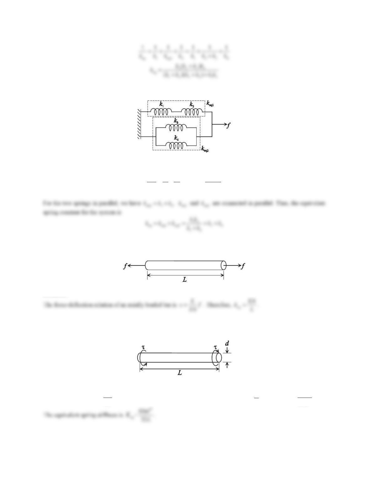
7. Determine the equivalent spring constant for the system shown in Figure 5.17.
Figure 5.17 Problem 7.
Solution
For the two springs in parallel, we have
eq1 2 3
kkk
. They are connected with another two springs in series. Thus,
the equivalent spring constant for the system is
138
8. Determine the equivalent spring constant for the system shown in Figure 5.18.
Figure 5.18 Problem 8.
Solution
For the two springs in series,
eq1 1 2
111
kkk
or
12
eq1
12
kk
kkk
9. Derive the spring constant expression for the axially loaded bar shown in Figure 5.19. Assume that the cross-
sectional area is A and the modulus of elasticity of the material is E.
Figure 5.19 Problem 9.
Solution
10. The uniform circular shaft in Figure 5.20 acts as a torsional spring. Assume that the elastic shear modulus of the
material is G. Derive the equivalent spring constant corresponding to a pair of torques applied at two free ends.
Figure 5.20 Problem 10.
Solution
For a shaft, we have
șIJ
L
GJ
, where the polar moment of inertia for a cylinder is
4
1
32
ʌJd
. Thus,
4
32
șIJ
ʌ
L
Gd
.
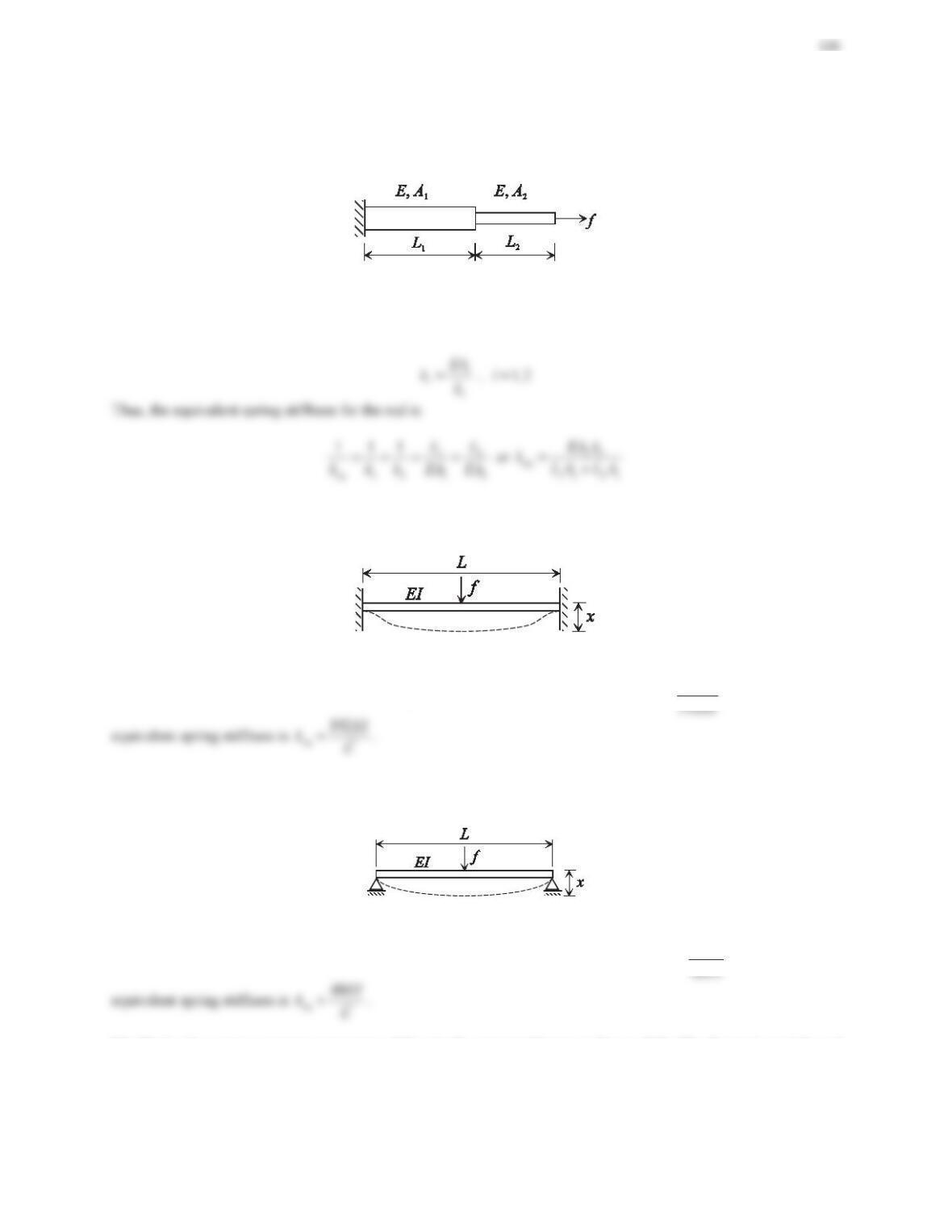
11. A rod is made of two uniform sections, as shown in Figure 5.21. The two sections are made of the same
material, and the modulus of elasticity of the rod material is E. The areas for the two sections are A1and A2,
respectively. Derive the equivalent spring constant corresponding to a tensile force applied at the free end.
Figure 5.21 Problem 11.
Solution
The rod with two uniform sections can be treated as two axial springs in series. Using the result obtained in Problem
9, the equivalent spring stiffness for each section is
12. Derive the spring constant expression of the fixed-fixed beam in Figure 5.22. The Young’s modulus of the
material is Eand the moment of inertia of cross-sectional area is I. Assume that the force fand the deflection x
are at the center of the beam.
Figure 5.22 Problem 12.
Solution
For a fixed-fixed beam with a load at midspan, the force-deflection relation is
3
L
xf
. Therefore, the
13. Derive the spring constant expression of the simply supported beam in Figure 5.23. The Young’s modulus of
the material is Eand the moment of inertia of cross-sectional area is I. Assume that the force fand the deflection
xare at the center of the beam.
Figure 5.23 Problem 13.
Solution
For a simply supported beam with a load at midspan, the force-deflection relation is
3
L
xf
. Therefore, the
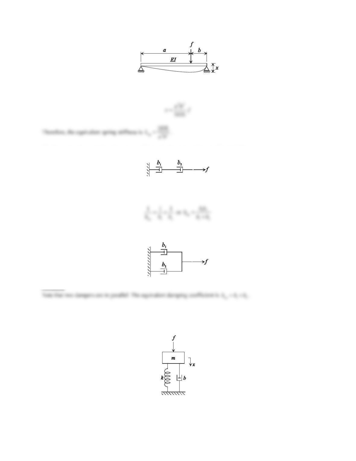
14. Derive the spring constant expression of the simply supported beam in Figure 5.24. The Young’s modulus of
the material is Eand the moment of inertia of cross-sectional area is I. Assume that the applied load fis
anywhere between the supports.
140
Figure 5.24 Problem 14.
Solution
For a simply supported beam with a load applied anywhere between supports, the force-deflection relation is
15. Determine the equivalent damping coefficient for the system shown in Figure 5.25.
Figure 5.25 Problem 15.
Solution
Note that two dampers are in series. The equivalent damping coefficient is
16. Determine the equivalent damping coefficient for the system shown in Figure 5.26.
Figure 5.26 Problem 16.
Problem Set 5.2
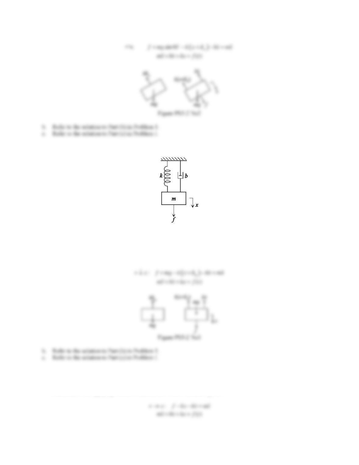
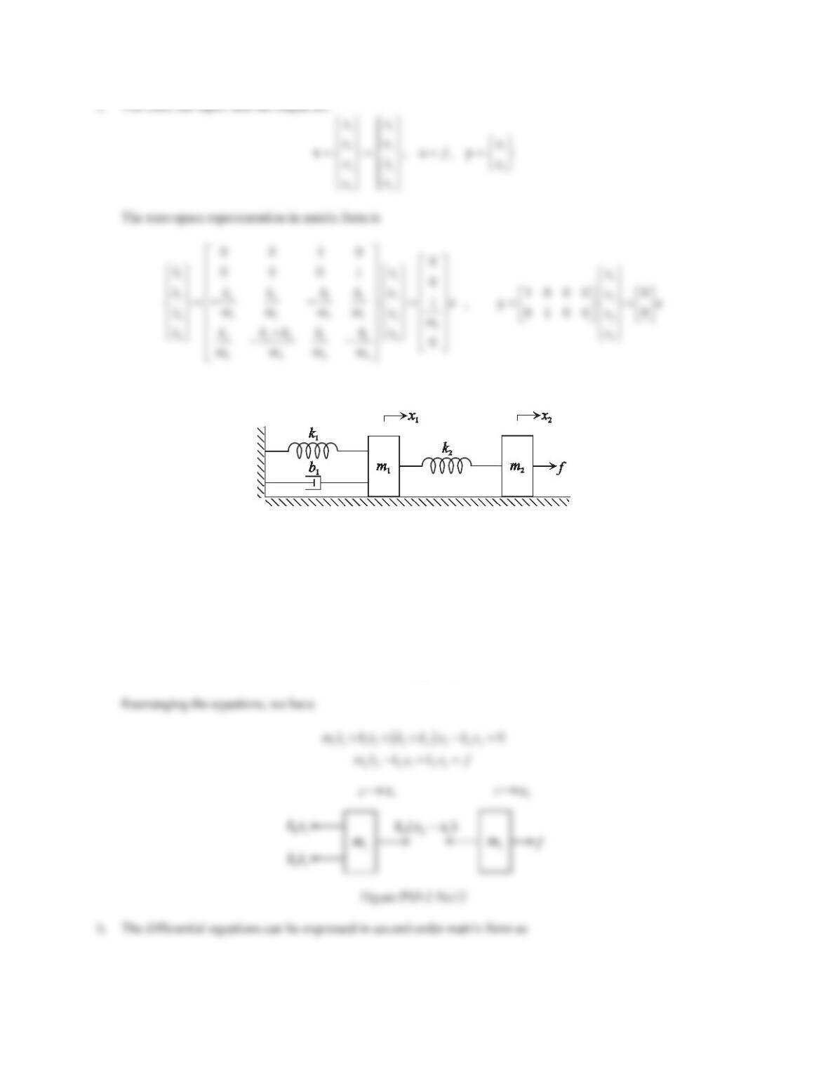
1. For the system shown in Figure 5.38, the input is the force fand the output is the displacement xof the mass.
Figure 5.38 Problem 1.
a. Draw the necessary free-body diagram and derive the differential equation of motion.
141
b. Using the differential equation obtained in Part (a), determine the transfer function. Assume initial
conditions x(0) = 0 and
(0) 0x
.
c. Using the differential equation obtained in Part (a), determine the state-space representation.
Solution
a. The free-body diagram is shown in the figure below. Due to gravity, the spring is compressed by
st
G
when the
mass is in static equilibrium and
st
mg k
G
. Choosing the static equilibrium as the origin of the coordinate
x
and applying Newton’s second law in the x–direction gives
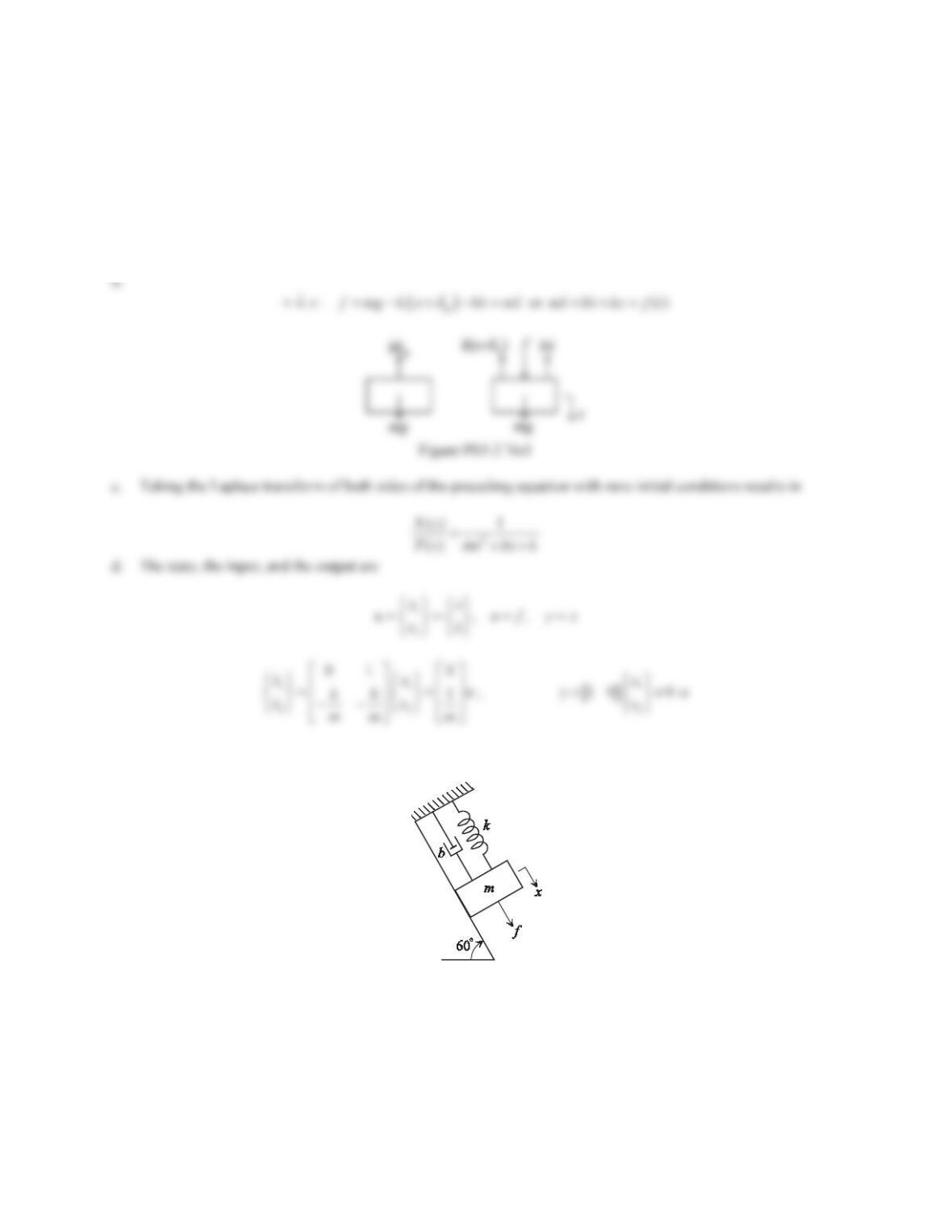
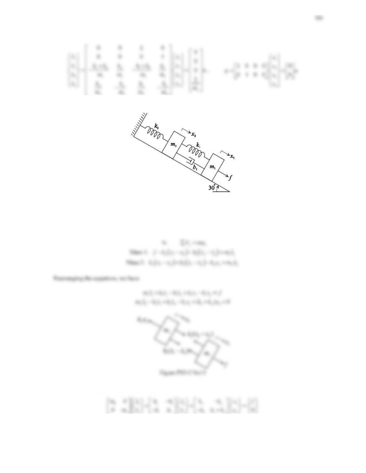
2. Repeat Problem 1 for the system shown in Figure 5.39.
Figure 5.39 Problem 2.
Solution
a. The free-body diagram is shown in the figure below. Due to gravity, the spring is stretched by
st
G
when the
mass is in static equilibrium and
st
sin 60mg k
G
D
. Choosing the static equilibrium as the origin of the
coordinate
x
and applying Newton’s second law in the x-direction gives
142
3. Repeat Problem 1 for the system shown in Figure 5.40.
Figure 5.40 Problem 3.
Solution
a. The free-body diagram is shown in the figure below. Due to gravity, the spring is stretched by
st
G
when the
mass is in static equilibrium and
st
mg k
G
. Choosing the static equilibrium as the origin of the coordinate xand
applying Newton’s second law in the x-direction gives
4. Repeat Problem 1 for the system shown in Figure 5.41.
Solution
a. The free-body diagram is shown in the figure below. Choosing the static equilibrium as the origin of the
coordinate xand applying Newton’s second law in the x-direction gives
143
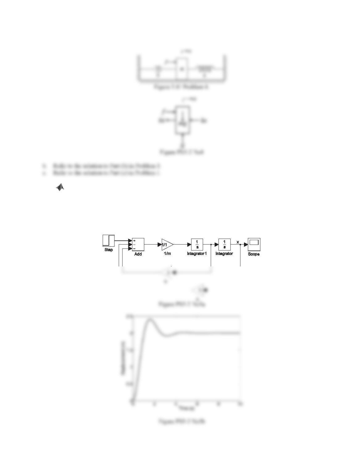
5. For Problems 1 through 4, use Simulinkto construct block diagrams to find the displacement output x(t)
of the system subjected to an applied force f(t) = 10u(t), where u(t) is the unit-step function. The parameter
values are m= 1 kg, b= 2 N·s/m, and k= 5 N/m. Assume zero initial conditions.
Solution
Since the systems in Problem 1 through 4 have the same mathematical model, we can use the same Simulink block
diagram to find the displacement output.
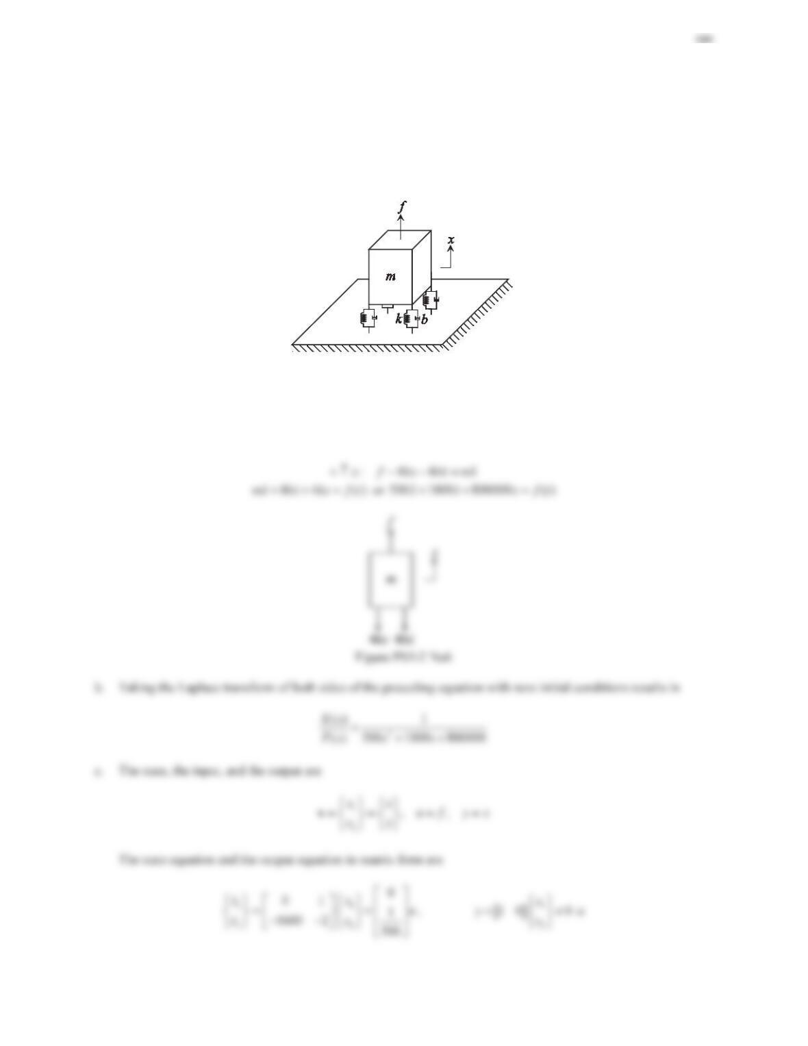
6. The system shown in Figure 5.42 simulates a machine supported by rubbers, which are approximated as four
same spring-damper units. The input is the force fand the output is the displacement xof the mass. The
parameter values are m= 500 kg, b= 250 N·s/m, and k= 200,000 N/m.
a. Draw the necessary free-body diagram and derive the differential equation of motion.
b. Determine the transfer function form. Assume zero initial conditions.
c. Determine the state-space representation.
d. Find the transfer function from the state-space form and compare with the result obtained in Part (b).
Figure 5.42 Problem 6.
Solution
a. The free-body diagram is shown in the figure below. Note that four same spring-damper units are connected in
parallel. Therefore, the equivalent spring stiffness is 4kand the equivalent damping coefficient is 4b.Let us
choose the static equilibrium as the origin of the coordinate x. Then, the static spring force will be cancelled by
the weight. Applying Newton’s second law in the x-direction gives
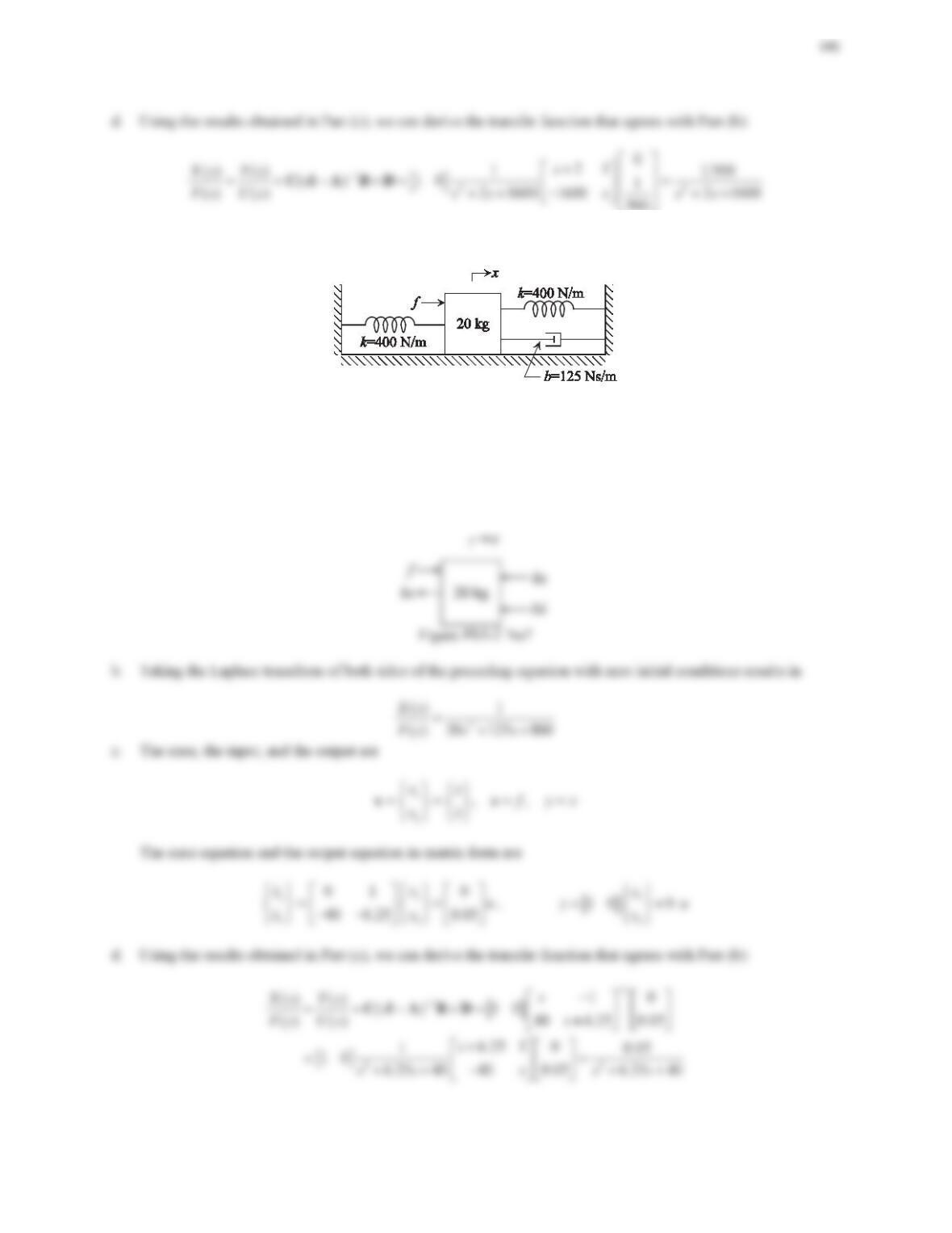
7. Repeat Problem 6 for the system shown in Figure 5.43.
Figure 5.43 Problem 7.
Solution
a. The free-body diagram is shown in the figure below. Choosing the static equilibrium as the origin of the
coordinate xand applying Newton’s second law in the x-direction gives
:2xfkxbxmxo
2()mx bx kx f t
or
20 125 800 ( )xxxft
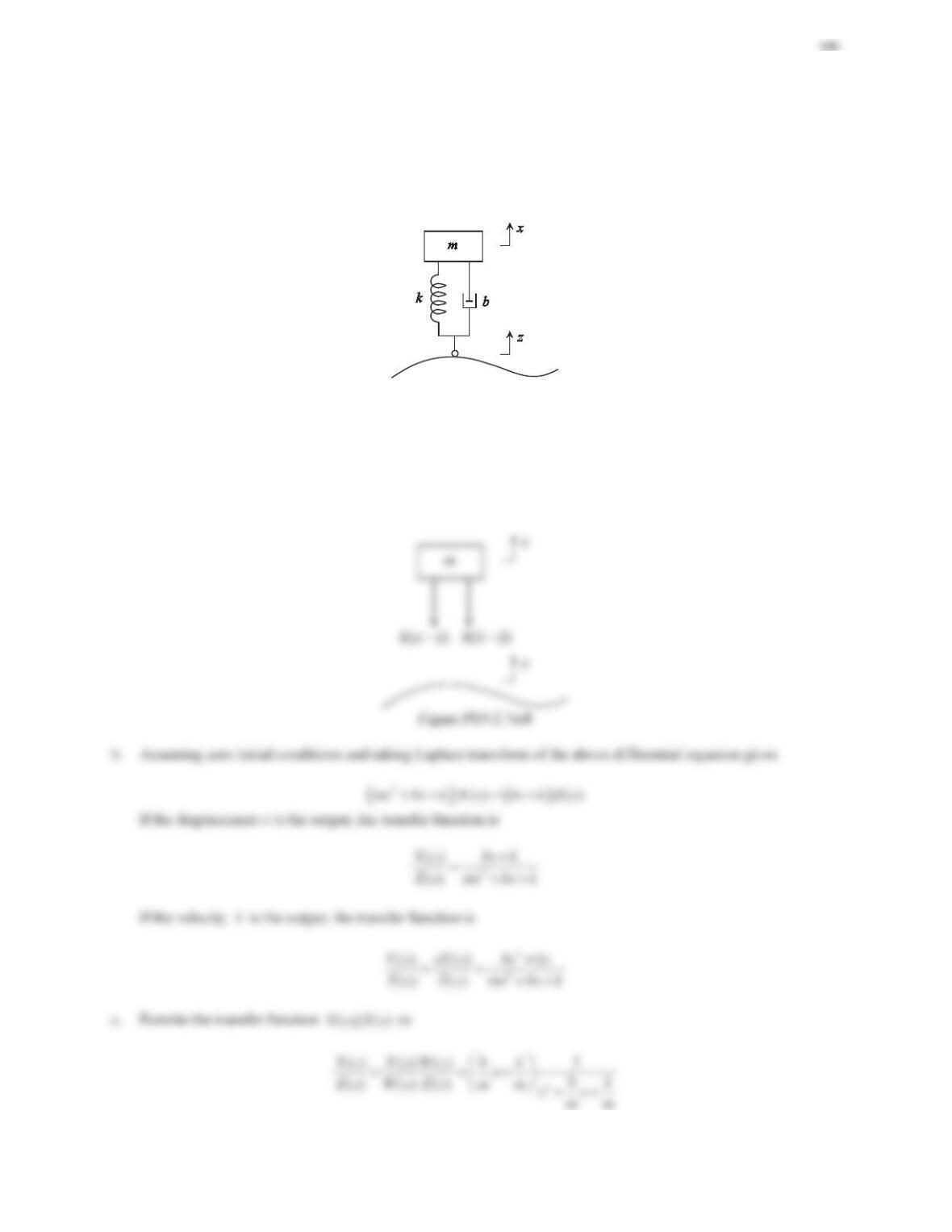
8. The system shown in Figure 5.44 simulates a vehicle traveling on a rough road. The input is the displacement z.
a. Draw the necessary free-body diagram and derive the differential equation of motion.
b. Assuming zero initial conditions, determine the transfer function for two different cases of output: (1)
displacement xand (2) velocity
x
.
c. Determine the state-space representation for two different cases of output: (1) displacement xand (2)
velocity
x
.
Figure 5.44 Problem 8.
Solution
a. We choose the static equilibrium as the origin of the coordinate x. Then, the static spring force will be cancelled
by the weight. Assume that 0xz!!. Applying Newton’s second law in the x-direction gives
:xkxzbxzmxn
mx bx kx bz kz
147
where
()
()
Xs b k
s
Ws m m
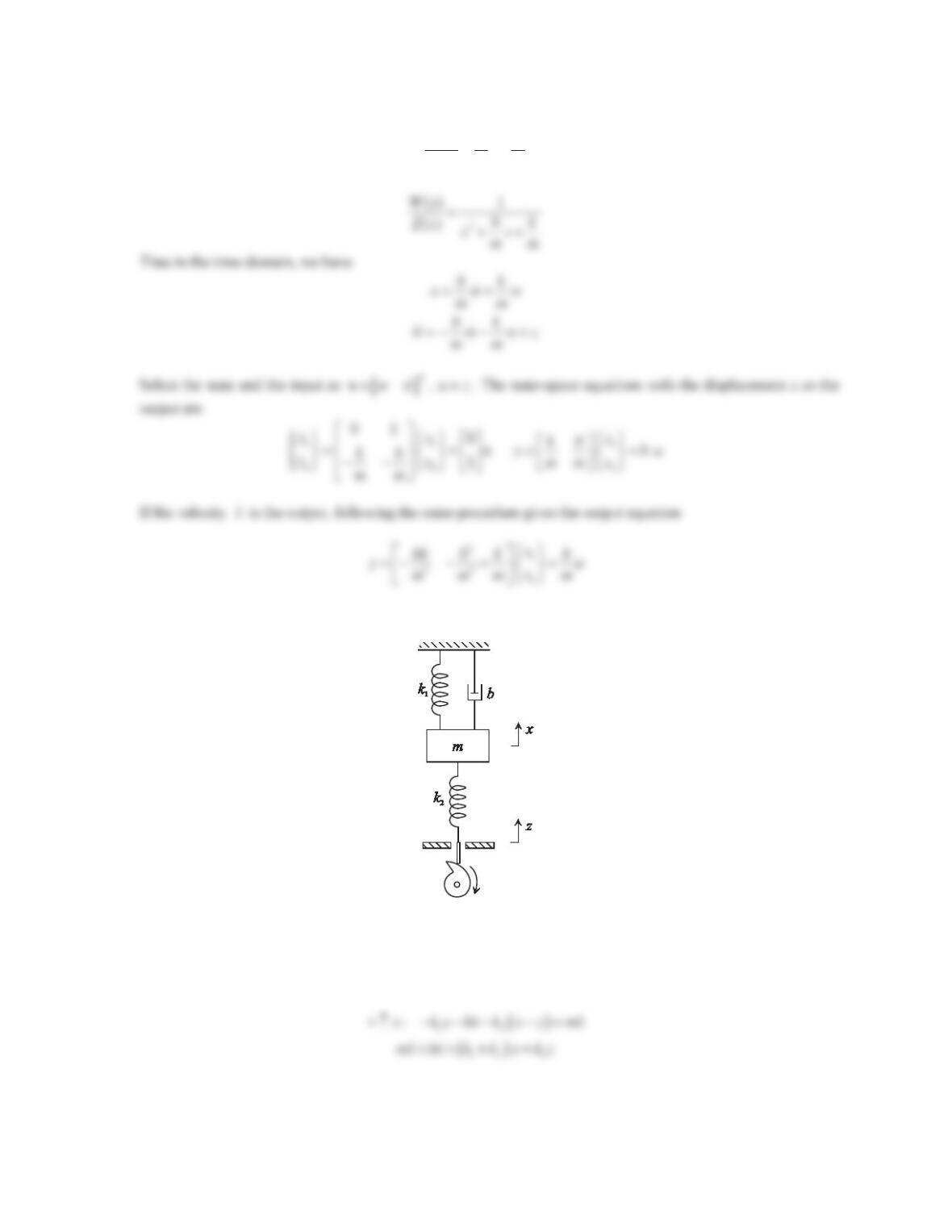
9. Repeat Problem 8 for the system shown in Figure 5.45, where the cam and follower impart a displacement zto
the lower end of the system.
Figure 5.45 Problem 9.
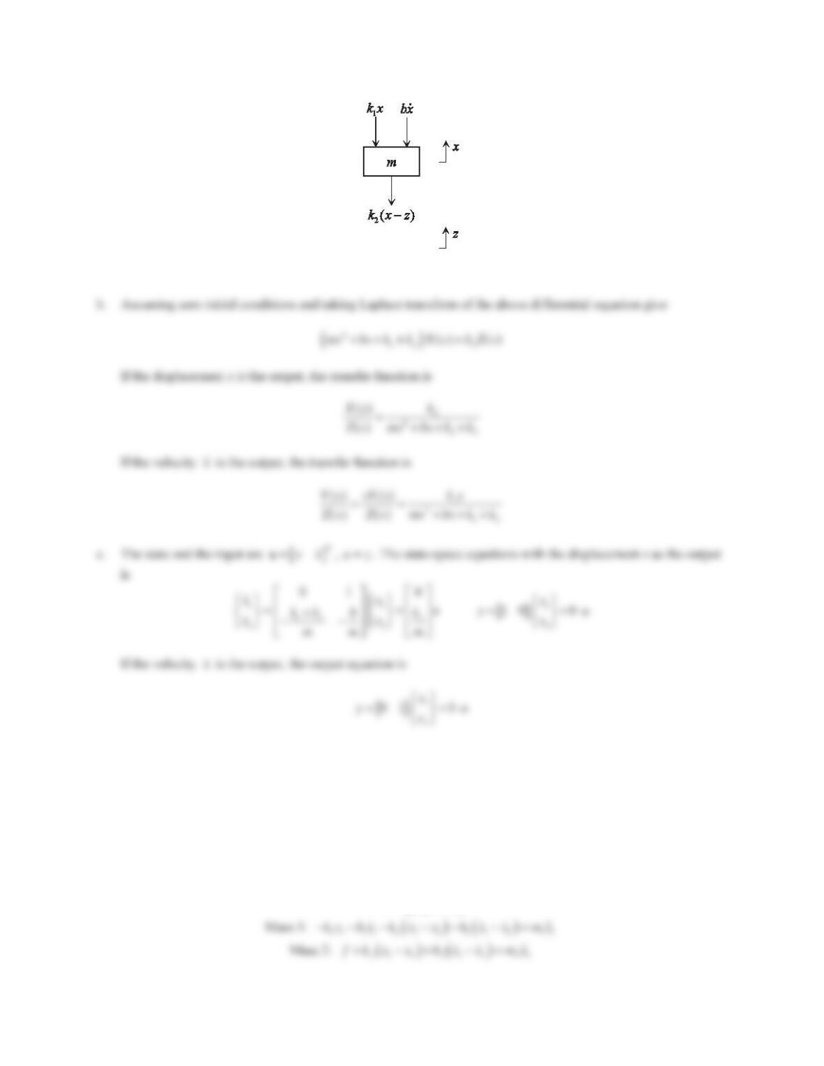
Solution
a. We choose the static equilibrium as the origin of the coordinate x. Then, the static spring force will be cancelled
by the weight Assume that 0xz!!. The free-body diagram is shown in the figure below. Applying Newton’s
second law in the x-direction gives
148
Figure PS5-2 No9
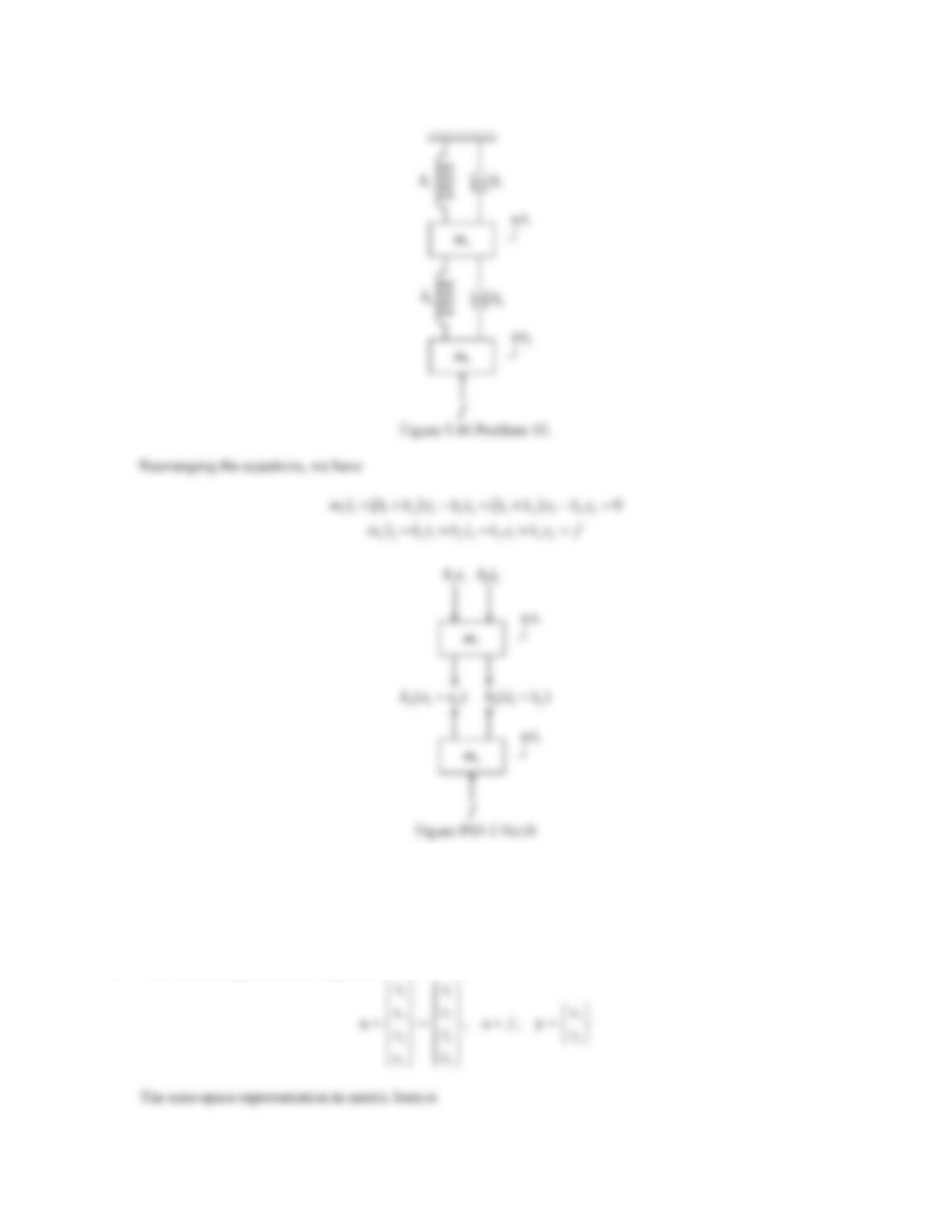
10. For the system shown in Figure 5.46, the input is the force fand the outputs are the displacements x1and x2of
the masses.
a. Draw the necessary free-body diagrams and derive the differential equations of motion.
b. Write the differential equations of motion in the second-order matrix form.
c. Using the differential equations obtained in Part (a), determine the state-space representation.
Solution
a. We choose the displacements of the two masses
1
x
and 2
xas the generalized coordinates. The static
equilibrium positions of
1
m
and
2
m
are set as the coordinate origins. Assume that
12
0xx!!
. Applying
Newton’s second law in the x-direction gives
:
xx
xFman ¦
149
b. The differential equations can be expressed in second-order matrix form as
1 1 12 21 12 21
22 2 2 2 2 2 2
00
0
mxbbbxkkkx
mx b b x k k x f
½ ½ ½
ªºª ºª º½
®¾ ®¾ ®¾®¾
«»« »« »
¯¿
¯¿ ¯¿ ¯¿
¬¼¬ ¼¬ ¼
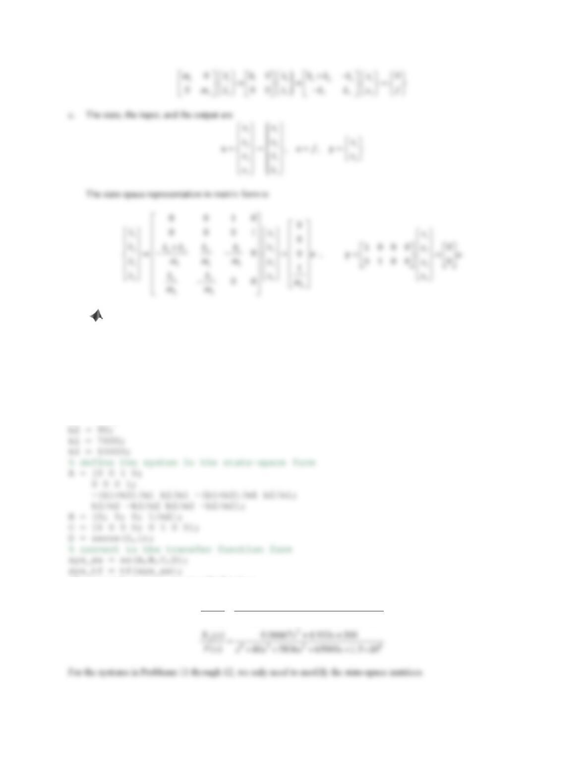
c. The state, the input, and the output are
11. Repeat Problem 10 for the system shown in Figure 5.47.
Figure 5.47 Problem 11.
Solution
a. We choose the displacements of the two masses
1
x
and 2
xas the generalized coordinates. The static
equilibrium positions of
1
m
and
2
m
are set as the coordinate origins. Assume that
12
0xx!!
. Applying
Newton’s second law in the x-direction gives
b. The differential equations can be expressed in second-order matrix form as
151
12. Repeat Problem 10 for the system shown in Figure 5.48.
Figure 5.48 Problem 12.
Solution
a. We choose the displacements of the two masses
1
x
and 2
xas the generalized coordinates. The static
equilibrium positions of
1
m
and
2
m
are set as the coordinate origins. Assume that
21
0xx!!
. Applying
Newton’s second law in the x-direction gives
:
xx
xFmao ¦
Mass 1:
11 11 2 2 1 11
kx bx k x x mx
Mass 2:
22 1 22
fkx x mx
152
13. For Problems 10 through 12, use MATLAB commands to define the systems in the state-space form and
then convert to the transfer function form. Assume that the displacements of the two masses, x1and x2, are the
outputs, and all initial conditions are zero. The masses are m1= 5 kg and m2= 15 kg. The spring constants are k1
= 7.5 kN/m and k2= 15 kN/m. The viscous damping coefficients are b1= 280 N·s/m and b2= 90 N·s/m.
Solution
For the system in Problem 10, the MATLAB session is
% define the system parameters
m1 = 5;
m2 = 15;
b1 = 280;
The command tf returns two transfer functions
1
43 2 6
( ) 1.2 200
() 80 5836 65000 1.5 10
Xs s
Fs ss s s
u
153
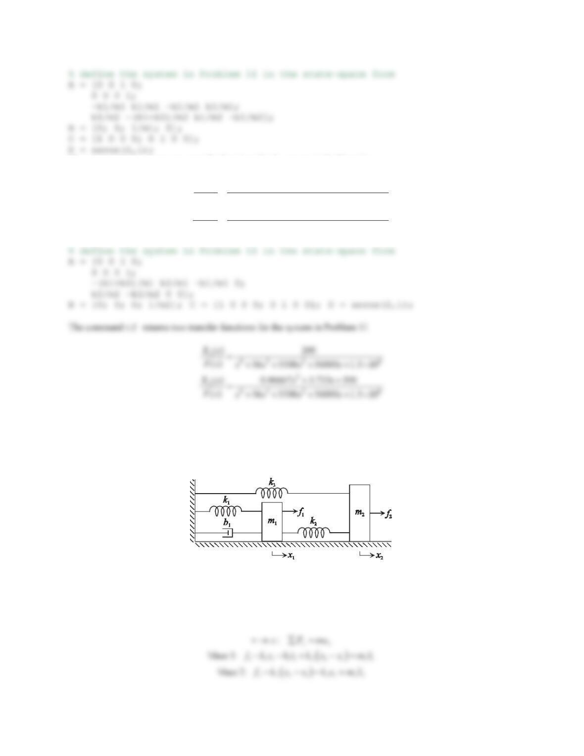
The command tf returns two transfer functions for the system in Problem 11
2
1
432 6
2
432 6
( ) 0.2 3.733 300
() 74.67 3000 56000 1.5 10
( ) 3.733 100
() 74.67 3000 56000 1.5 10
Xs s s
Fs sss s
Xs s
Fs sss s
u
u
14. For the system in Figure 5.49, the inputs are the forces f1and f2applied to the masses and the outputs are the
displacements x1and x2of the masses.
a. Draw the necessary free-body diagrams and derive the differential equations of motion.
b. Write the differential equations of motion in the second-order matrix form.
c. Using the differential equations obtained in Part (a), determine the state-space representation.
Figure 5.49 Problem 14.
Solution
a. We choose the displacements of the two masses
1
x
and 2
xas the generalized coordinates. The static
equilibrium positions of
1
m
and
2
m
are set as the coordinate origins. Assume that
21
0xx!!
. Applying
Newton’s second law in the x-direction gives