1
Review Problems
1. Write a user-defined function with function call C=temp_conv(F) that converts the temperature from
Farenheit Fto Celsius C. Execute the function for the case of F = 86.
Solution
function C = temp_conv(F)
C = (F-32)*100/180;
2. Write a user-defined function with function call [P A]=circ(r) that computes the perimeter Pand area Aof
a circle of radius r. Execute the function to calculate the perimeter and area of a circle with radius r=1.70.
Solution
function [P A] = circ(r)
3. Write a user-defined function with function call val=evalf(f,a,b) where fis an inline function, and a
and bare constants such that
ab
. The function calculates the midpoint
m
of the interval
>@
,ab
and returns
the value of
11 1
23 4
() ( ) ()fa fm fb
. Execute the function for
() cos2
x
fx e x
,
1a
,
3b
.
Solution
4. Write a user-defined function with function call Q = laplace_eval(f,a,b) where fis a function
defined symbolically, and aand bare constants. The function calculates
xx yy
ff
, and evaluates the result at
xa
,
yb
. Execute the function for
2
cos 1/fx y y
,0a ,
1b
.
2
5. Write a user-defined function with function call P=partial_eval(f,g,a) where fand gare functions
defined symbolically, and ais a constant. The function returns the value of
fg
cc
at
xa
. Execute the
function for
2/3x
fxe
,
cosgx
, and
0.65a
.
Solution
6. Write a user-defined function with function call m=mid_point(a,b,e) where aand bare constants, and e
is a tolerance. The function calculates the midpoint of
>@
,ab
, called
1
m
, then the midpoint of
>@
1
,am
, called
2
m
, then the midpoint of
>@
2
,am
, called
3
m
, and so on. The process terminates when
1kk
mm e
is met.
Allow a maximum of 20 iterations. The function output will be the sequence of generated midpoints
1
m
,
2
m
,
… . Execute the function for the case of
1a
,
8b
, and
2
10e
(in MATLAB, written as 1e-2).
Solution
function m = mid_point(a,b,e)
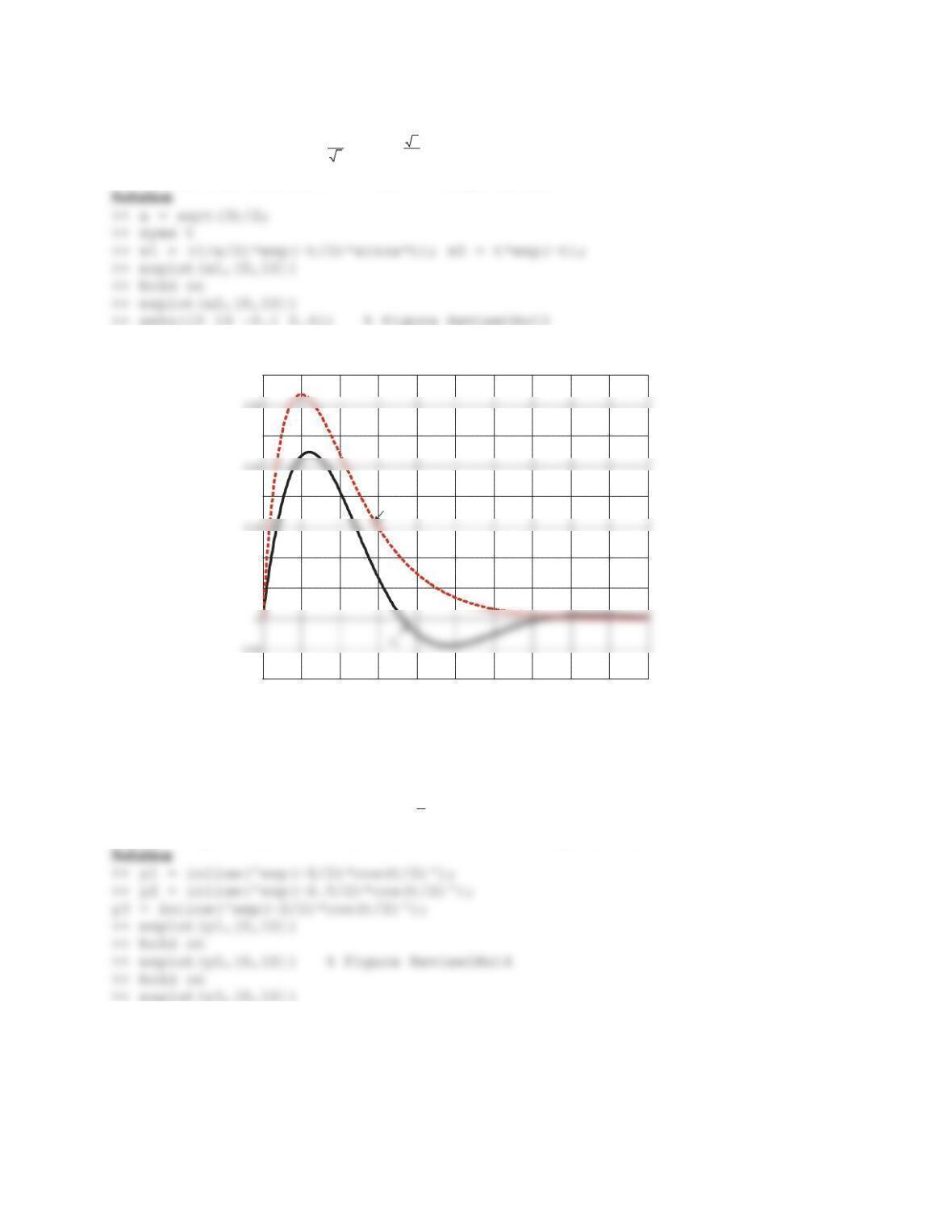
7.Plot
1
3
0
sin
txt
exdx
³
versus
0.1 7tdd
.
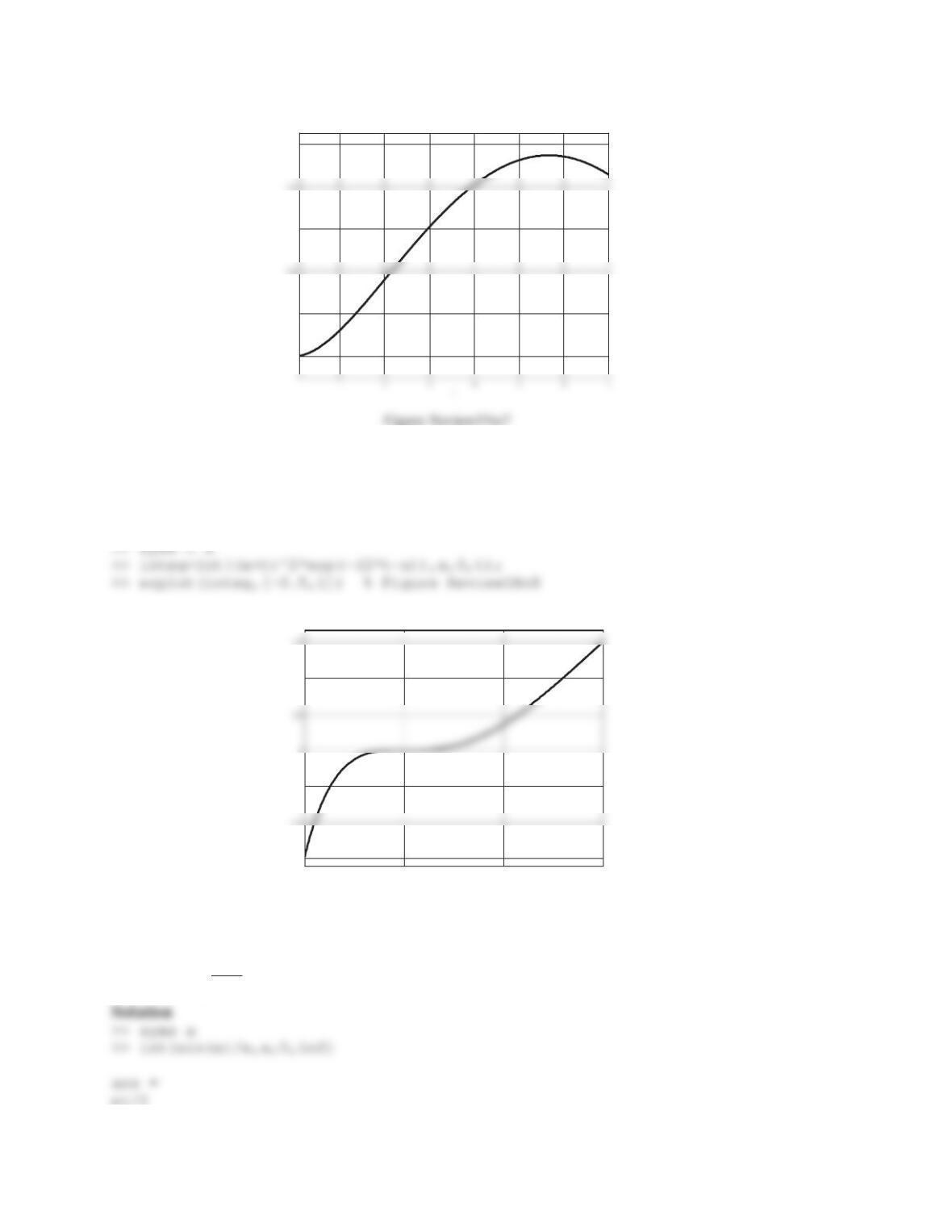
3
8. Plot
2(2)
0
()
ttx
xte dx
³
versus 0.5 1tdd
.
Solution
Figure Review1No8
9.Evaluate
0
sin xdx
x
f
³
.
0
0.2
0.6
1
-0.5 00.5 1
-0.6
-0.2
0.4
t
4
10. Differentiate
232
() 3 sin
xx
hx x e
with respect to
x
, and evaluate at
0.75x
.
Solution
>> syms x
9.3384
11. Write a script file that uses any combination of the flow control commands to generate
103000
020300
10 3 030
010403
00 1050
000 106
ªº
«»
«»
«»
«»
«»
«»
«»
«»
¬¼
A
Solution
A = zeros(6,6);
for i = 1:6,
12. Write a script file that uses any combination of the flow control commands to generate
41 32 0 0
04 13 2 0
00 4 1 32
00 0 4 13
00 0 0 4 1
00 0 0 0 4
ªº
«»
«»
«»
«»
«»
«»
«»
«»
¬¼
A
Solution
A = 4*eye(6);
for i = 1:6,
for j = 1:6,
5
13. Plot the two functions
/2 3
1
12
3
() sin
t
xt e t
and
2() t
xt te
versus
010tdd
in the same graph. Adjust
the limits of the vertical axis to 0.1and
0.4
. Add grid and label.
Figure Review1No13
14. Plot the three functions
/2 1
1,2,3 2
() cosyte t
D
, corresponding to
1, 1.5, 2
D
, versus
010tdd
in the same
graph. Adjust the limits of the vertical axis to
0.8
and
0.8
. Add grid and label.
0 1 2 3 4 5 6 7 8 9 10
-0.1
0.05
0.1
0.2
0.3
0.4
t
x
2
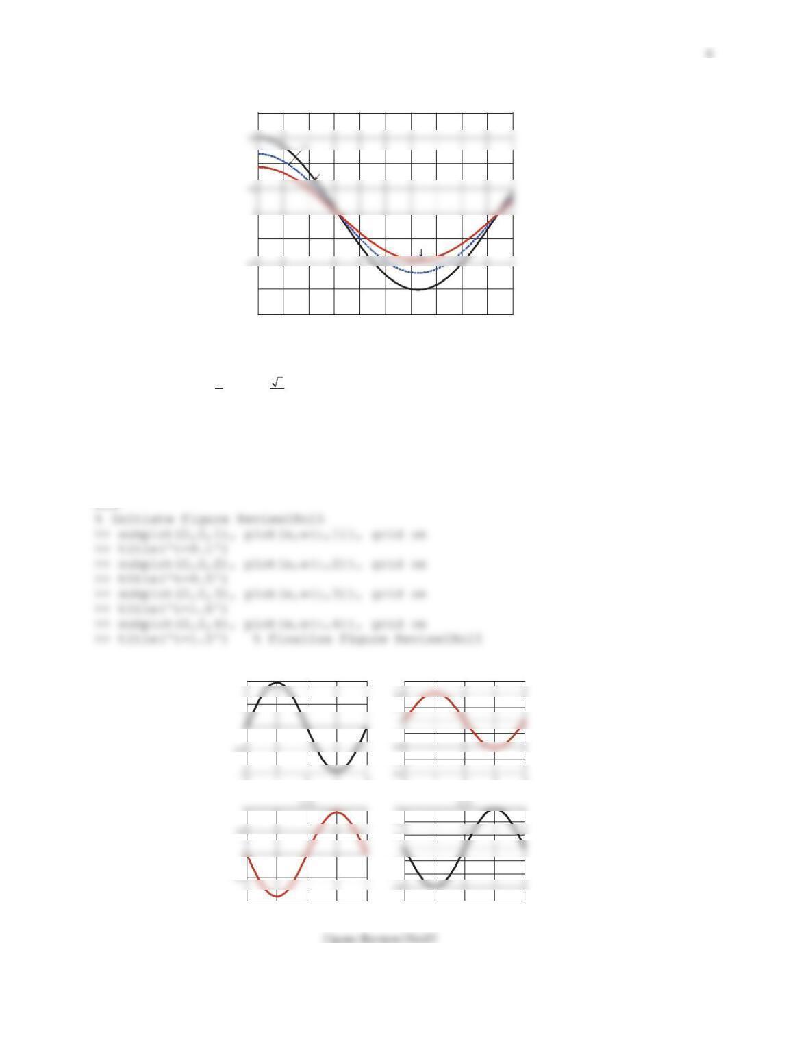
Figure Review1No14
15. Plot
3
1
22
(,) sin coswxt x t
SS
versus 04xdd for
0.1, 0.5, 1, 1.5t
in a
22u
tile and add title.
Solution
>> x = linspace(0,4); t = [0.1 0.5 1.0 1.5];
>> for i=1:4,
for j=1:100,
w(j,i)=sin(pi*x(j)/2)*cos(sqrt(3)/2*pi*t(i));
end
0 1 2345 6 7 8 9 10
-0.8
-0.6
-0.2
0.4
0.8
t
y
1
y
3
0.5
1
t=0.1
-0.3
-0.1
0.1
0.3
t=0.5
0 1 2 3 4
-1
0 1 2 3 4
-0.8
-0.4
-0.2
0.2
7
16. Plot
(1)
(,) 1 sin
t
uxt xe
versus 05xdd for
1, 2t
in a
12u
tile. Add grid and title.
Solution
x = linspace(0,5); t = [1,2];
Figure Review1No16
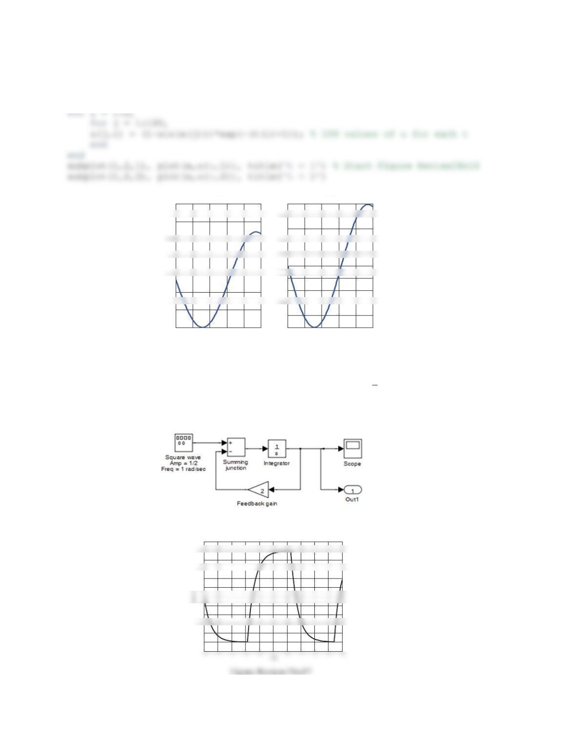
17. Create the Simulink model shown in Figure 1.22. Double clicking on each block allows you to explore its
properties. Choose the signal generator as a square wave with amplitude of
1
2
and frequency of 1 rad/sec. To
flip the gain block (Commonly Used Blocks), right click on it, then go to format and choose the “flip block”
option. Perform simulation and generate a figure that can be imported into a document.
Figure 1.22 Problem 17.
Solution
0 1 2 3 4 5
0
0.05
0.1
0.3
0.35
t = 1
0 1 2 3 4 5
0
0.01
0.03
0.04
0.05
0.08
0.1
t = 2
-0.25
-0.2
-0.1
-0.05
0.05
0.1
0.2
18. Repeat Problem 17 for the model shown in Figure 1.23, where the input signal is a sine wave. Note that double
clicking on the Sum [Commonly Used Blocks] allows control over the list of desired signs.
Figure 1.23 Problem 18.
Solution
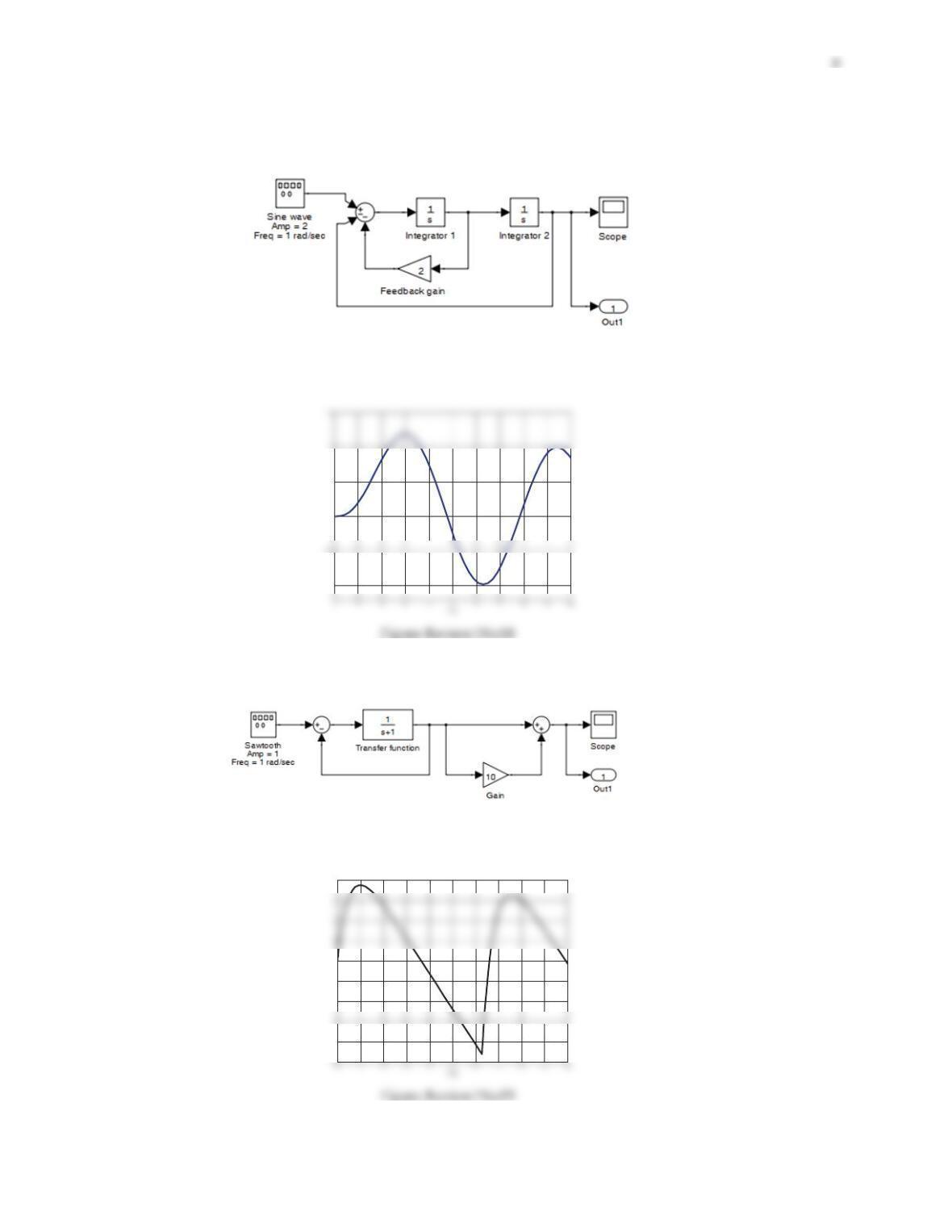
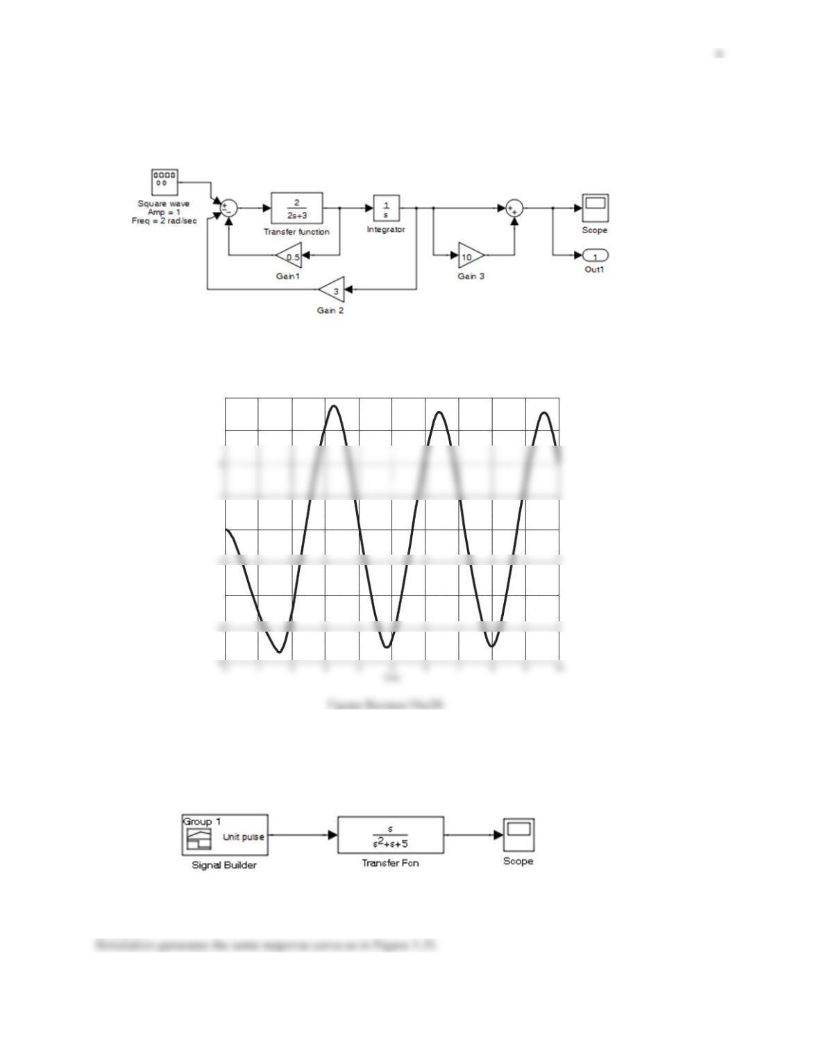
19. Build the model in Figure 1.24, perform simulation and generate a figure that can be imported into a document.
Figure 1.24 Problem 19.
Solution
-1
0
0.5
Response
-4
-2
-1
0
4
Response
20. Build the model shown in Figure 1.25, perform simulation, and generate a figure that can be imported into a
document.
Figure 1.25 Problem 20.
Solution
21. Figure 1.26 shows the Simulink model of the RLC circuit considered in this chapter and is equivalent to the
Simscape model presented in Figure 1.19. Perform the simulation to confirm that both models yield the same
response.
Figure 1.26 Problem 21.
Solution
-2
0
3
4
Response
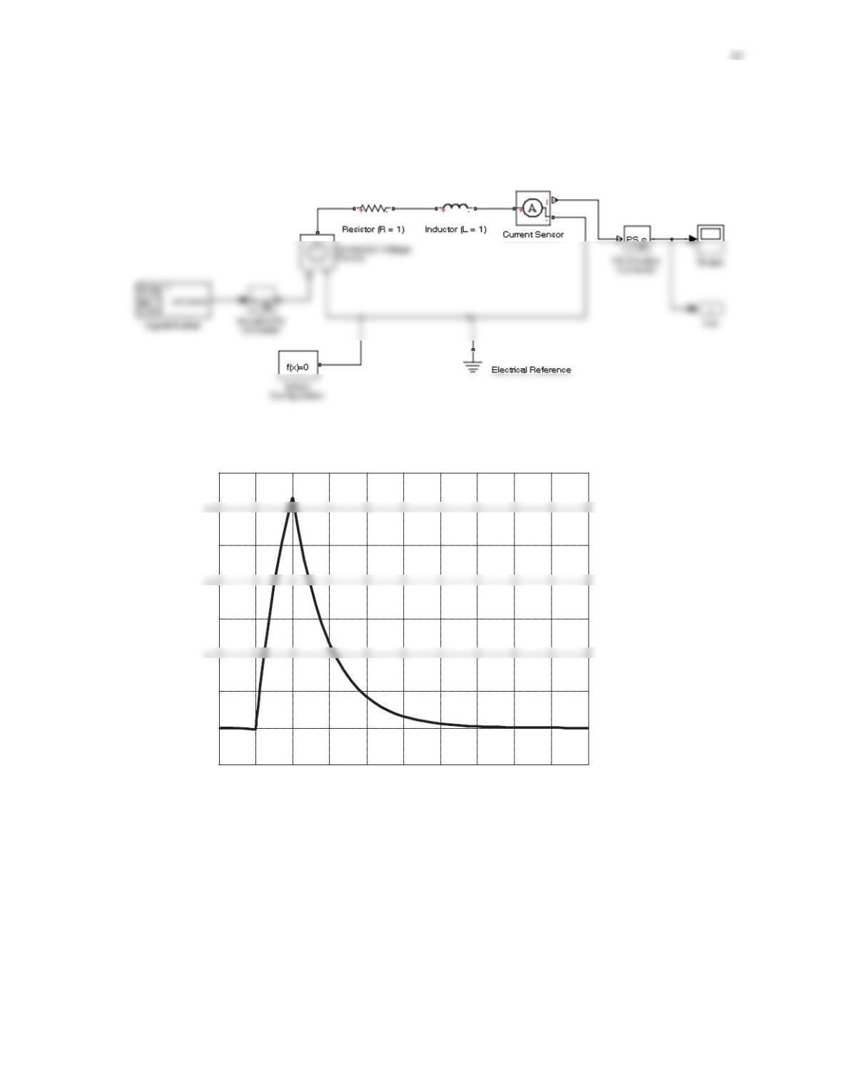
22. Consider an RL circuit with parameters and input signal identical to the RLC circuit considered in this chapter,
but with the capacitor removed. Build the Simscape model, run the simulation, and generate the response plot.
Solution
Figure Review1No22a
Figure Review1No22b
0 1 2 3 4 5 6 7 8 9 10
-0.05
0
0.05
0.15
0.25
0.35
Time
Current