459
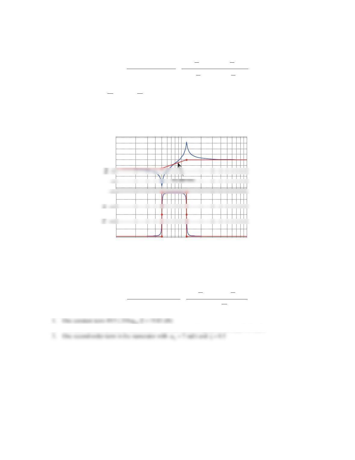
c. The frequency response function is
2
jȦMȦ
255
22
jȦMȦ
12 12
25 2 0.01 1
jȦ MȦ
(jȦ
jȦ MȦ 144 2 0.01 1
G
ªº
«»
¬¼
ªº
«»
¬¼
The basic terms include:
1. One constant term
25
144
(
25
10 144
20log 15
dB)
2. Two second-order terms: one in the numerator with
n
Ȧ
rad/s and
ȗ
and one in the denominator
with
n
Ȧ
rad/s and
ȗ
Bode Diagram
Frequency (rad/sec)
-30
-10
0
10
20
30
40
1 10 100
-360
-330
-270
-210
Figure PS10-6 No2c
d. The frequency response function is
2
2jȦMȦ
77
jȦ
500
49 2 0.5 1
100 jȦMȦ
(jȦ jȦ MȦ 5jȦ
G
ªº
ªº
«»
¬¼¬ ¼
The basic terms include:
2. Two first-order terms in the denominator with the corner frequencies at 1 and 500 rad/s
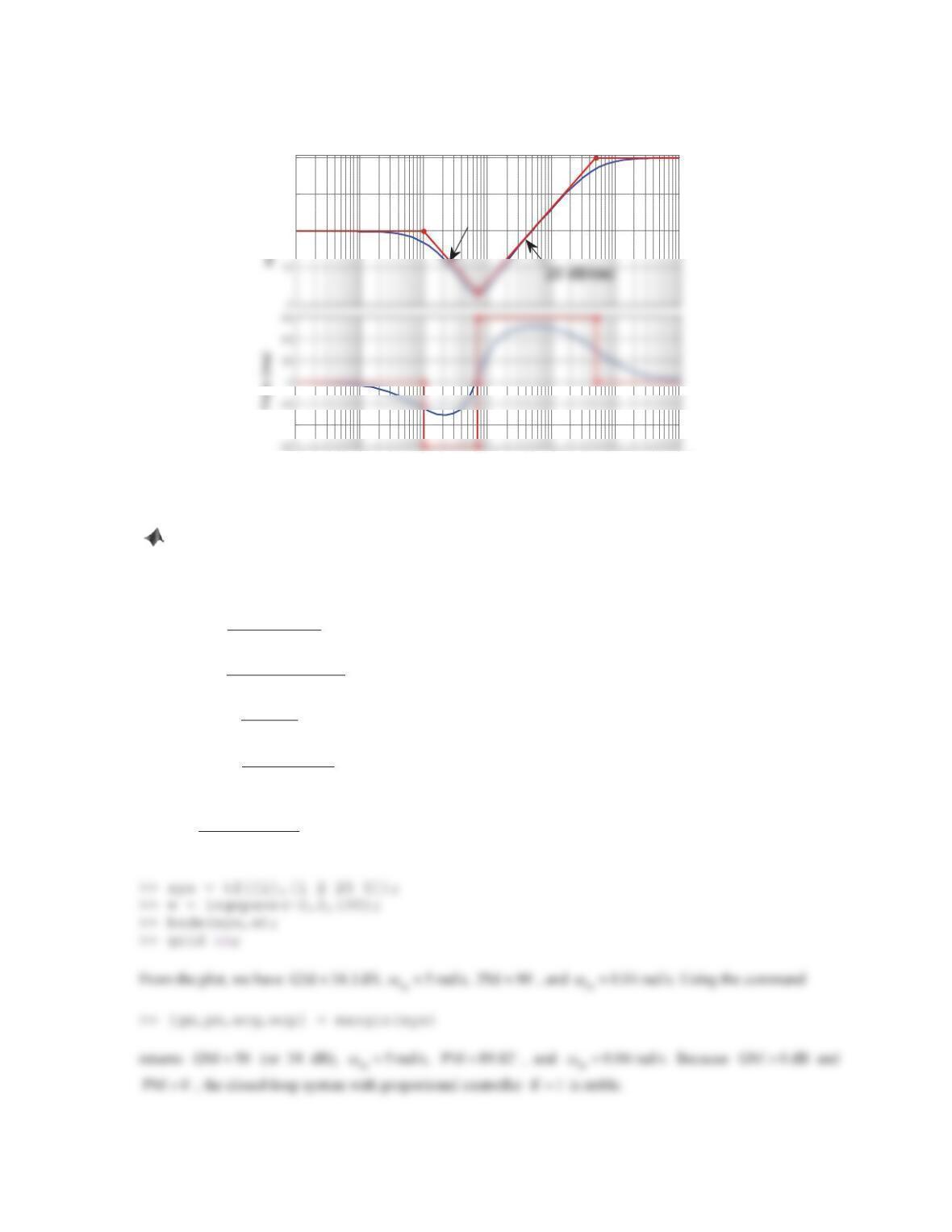
460
Bode Diagram
Frequency (rad/sec)
20
30
40
0.01 0.1 1 10 100 1000 10000
-60
-20 dB/dec
Figure PS10-6 No2d
3. For each of the following open-loop transfer functions, construct a Bode plot for K= 1 using the
MATLAB command bode. Estimate the GM, PM, and their associated crossover frequencies from the plot.
Verify the results using the MATLAB command margin. Determine the stability of the corresponding closed-
loop system.
a.
2
() ( 2 25)
K
KG s ss s
b. 2
100
() (4)( 22)
K
KG s sss
c.
2
0.5
() (2)
s
KG s K ss
d.
2
1
() ( 10)( 1)
KG s K ss
Solution
a.
22
() 225
K
KG s ss s
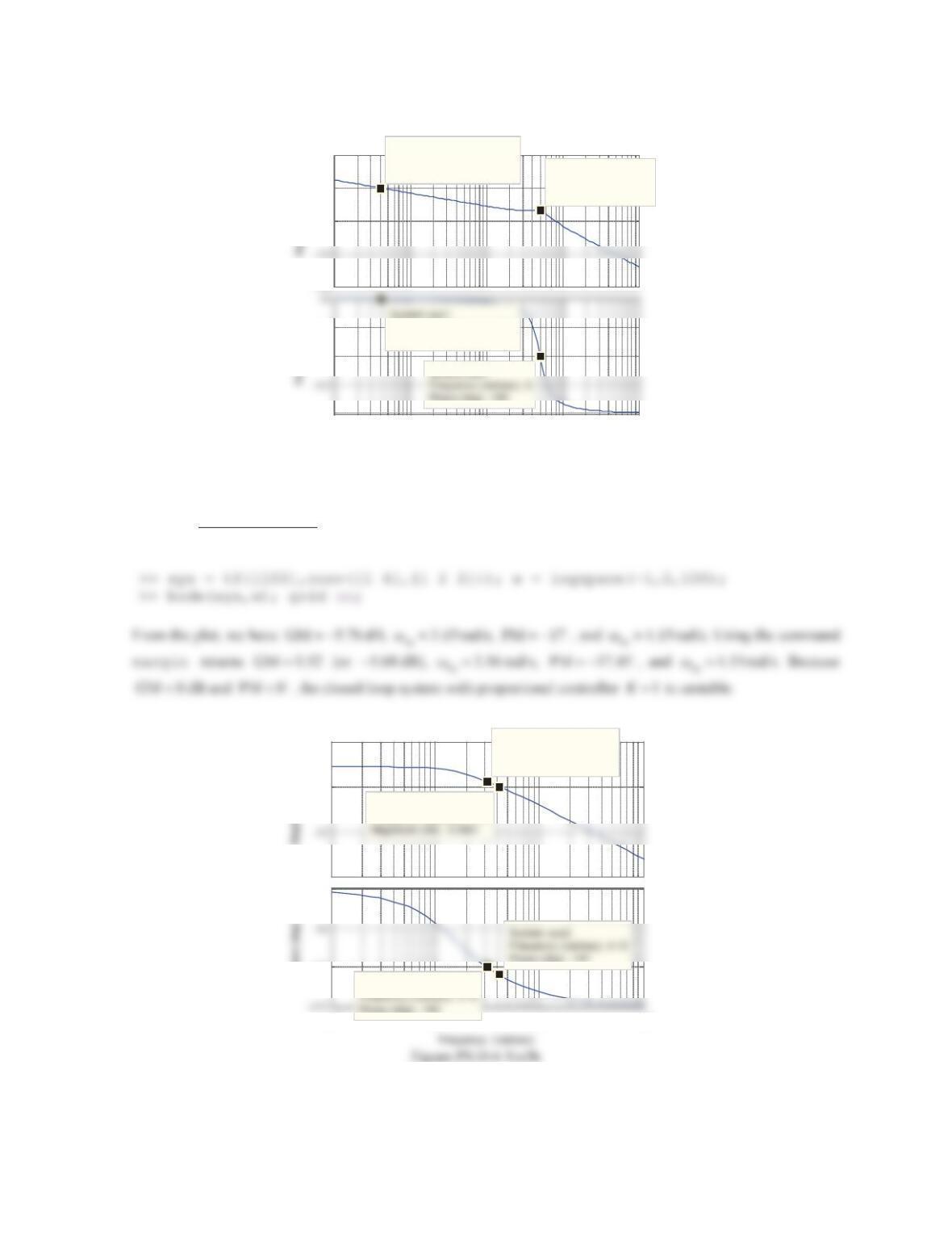
461
Bode Diagram
Frequency (rad/sec)
-50
0
50 System: sys1
Frequency (rad/sec): 0.0401
Magnitude (dB): –0.0119 System: sys1
Frequency (rad/sec): 5
Magnitude (dB): –34.1
10-2 10-1 100101102
–270
–180
–135
Frequency (rad/sec): 0.0401
Phase (deg): –90.2
Figure PS10-6 No3a
b.
2
100
() (4)( 22)
K
KG s sss
Bode Diagram
–100
0
50
System: sys2
Frequency (rad/sec): 4.15
System: sys2
Frequency (rad/sec): 3.15
Magnitude (dB): 5.76
10
-1
10
0
10
1
10
2
–180
0
System: sys2
Phase (deg)
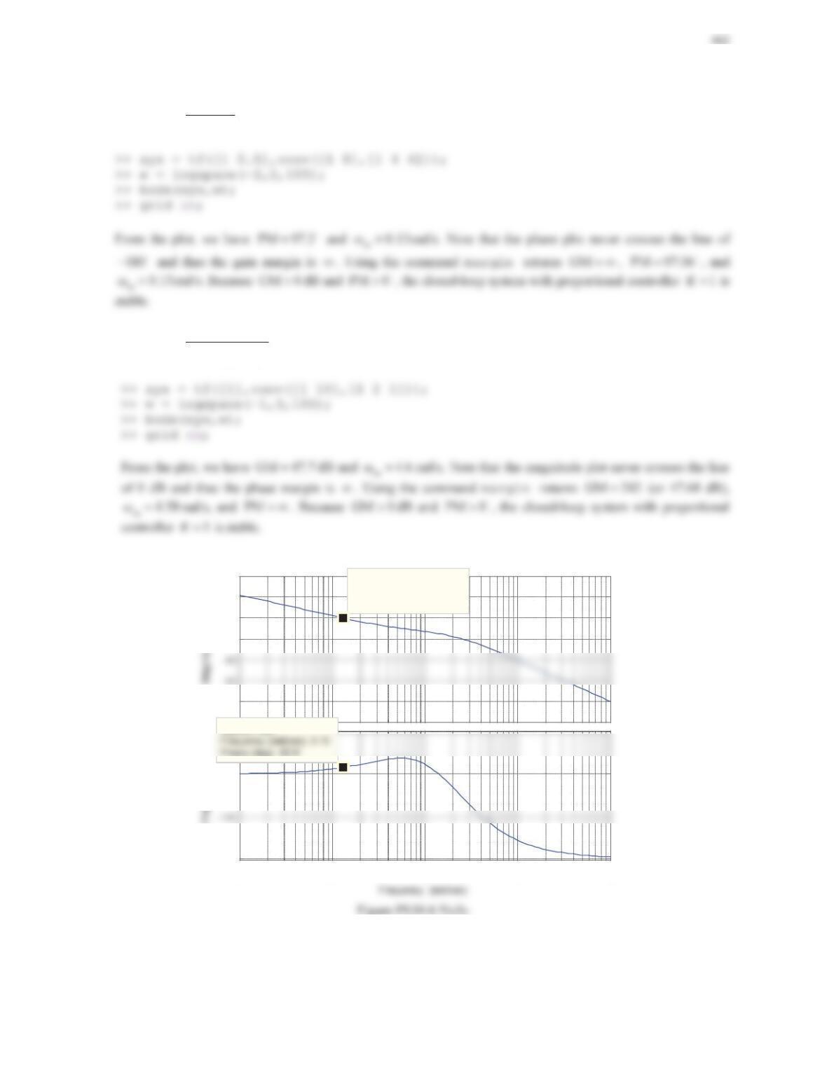
c.
2
0.5
() (2)
s
KG s K ss
d.
2
1
()
10 1
KG s K
ss
Bode Diagram
-100
-80
-20
0
20
40 System: sys
Frequency (rad/sec): 0.13
Magnitude (dB): -0.0704
10
-2
10
-1
10
0
10
1
10
2
-180
-90
System: sys
Frequency (rad/sec)
10
-1
10
0
10
1
10
2
10
3
–180
-90
Frequency (rad/sec): 4.6
Phase (deg): –180
Phase (deg)
–200
–100
-50
Magnitude (dB): –47.7
Figure PS10-6 No3d
4. Reconsider Problem 3. Each plant G(s) is controlled by a proportional controller Kvia unity negative
feedback. Determine the stability range of Kby sliding the magnitude plot up or down until instability occurs.
Verify the results by sketching a root locus.
Solution
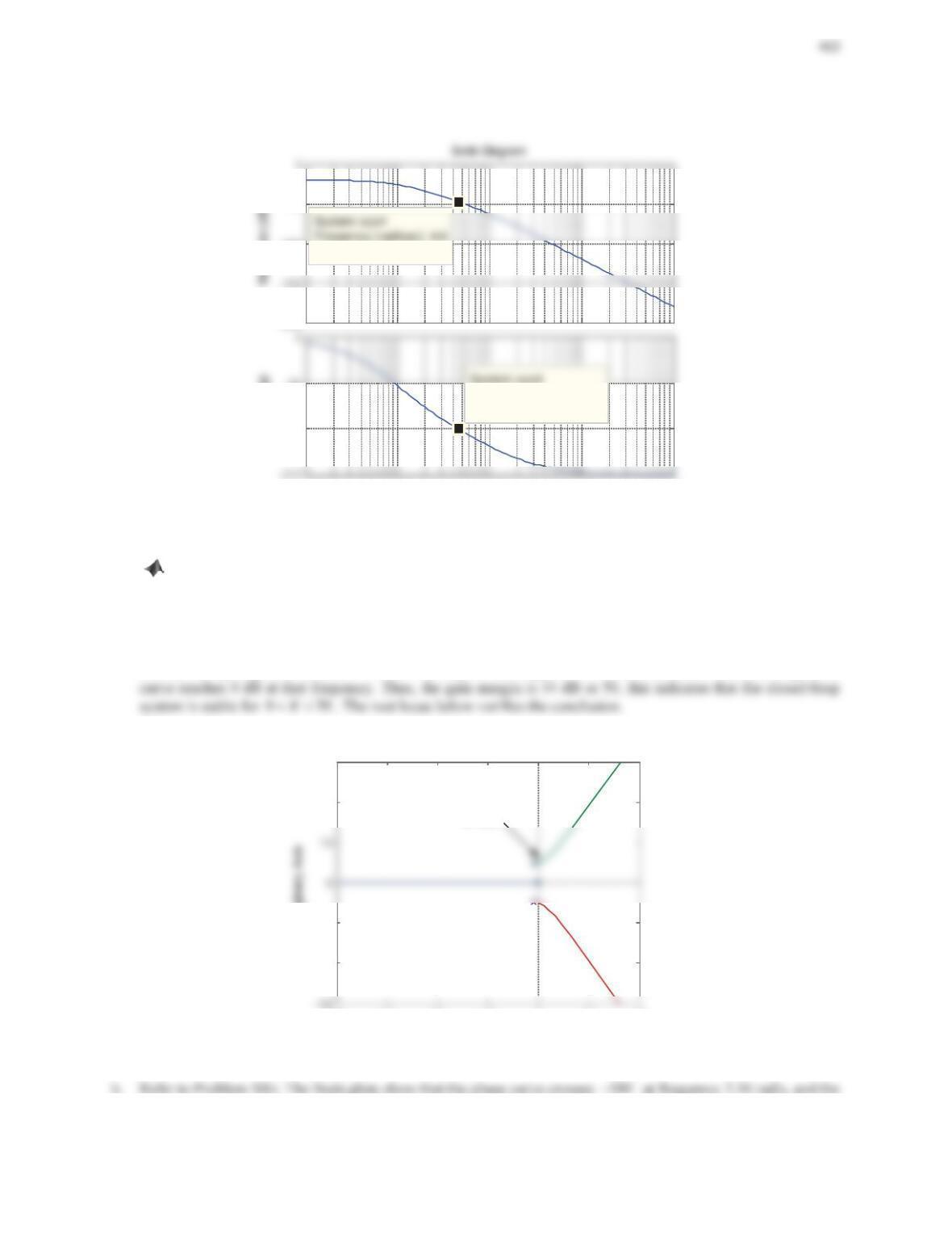
a. Refer to Problem 3(a). The Bode plots show that the phase curve crosses
180
D
at frequency 5 rad/s, and the
corresponding magnitude is about
34
dB. This implies that a gain of 34 dB can be added before the magnitude
-40 -30 -20 -10 010 20
-20
-10
20
30
Root Locus
R
ea
l Axi
s
Imaginary Axis
K=50
Figure PS10-6 No4a
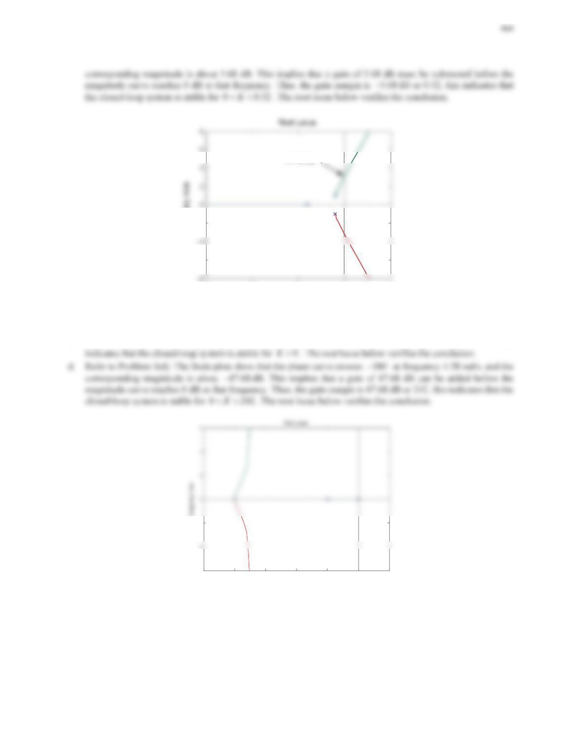
-15 -10 -5 0 5
-6
-2
R
ea
l Axi
s
Imaginary Axis
K=0.52
Figure PS10-6 No4(b)
c. Refer to Problem 3(c). The phase plot never crosses the line of
180
D
and thus the gain margin is f. This
-2.5 -2 -1.5 -1 -0.5 00.5
-6
-2
Real Axis
Figure PS10-6 No4(c)
-30 -20 -10 010
-30
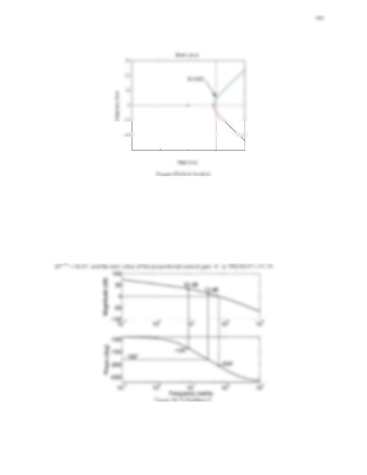
5. Figure 10.75 shows the Bode plot for an open-loop transfer function KG(s) with K= 500.
a. Determine the stability of the closed-loop system with K= 500.
b. Determine the value of Kthat would yield a PM of 45°.
Solution
a. As shown in the figure, the magnitude is 13 dB when the phase curve crosses
180D
. This implies that
GM 13 dB. The phase is
204D
when the magnitude curve crosses 0 dB. This implies that
PM 24 D
.
Because
GM 0
dB and
PM 0
D
, the closed-loop system with a proportional controller 500K is unstable.
b. To yield a phase margin of
45
D
, the phase when the magnitude plot crosses 0 dB should be
135
D
. It is
observed from the figure that the magnitude is 33 dB when the phase is
135
D
. To make the magnitude be 0
dB, the magnitude plot should slide downward by 33 dB. This is the effect of dividing by a constant term of
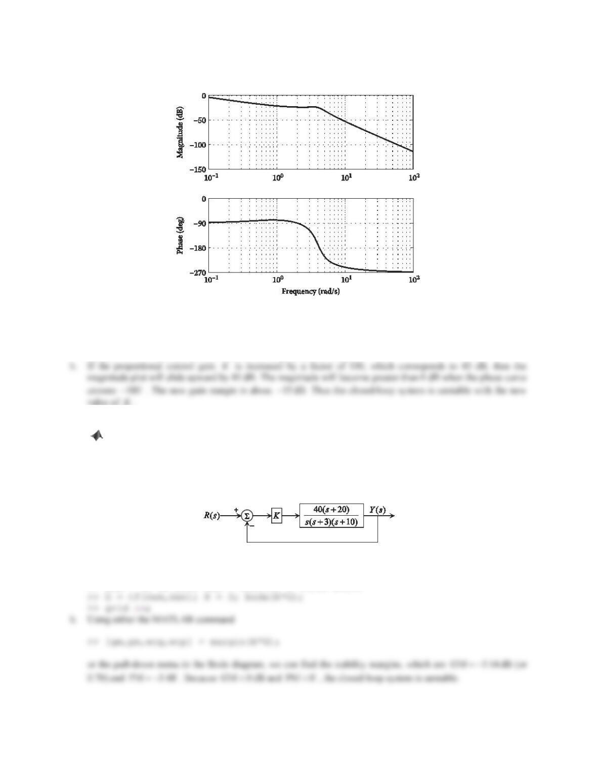
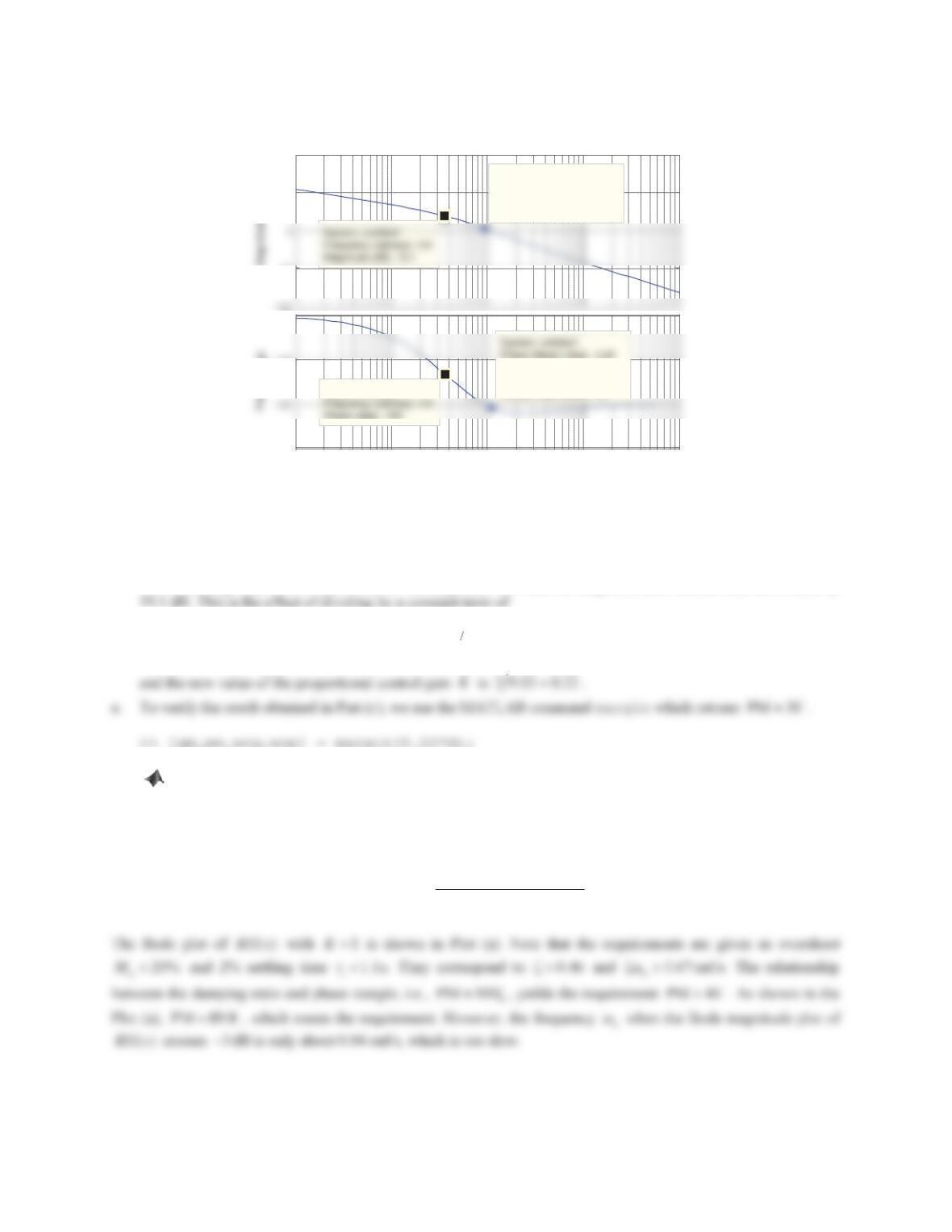
6. The Bode plot for an open-loop transfer function KG(s) is shown in Figure 10.76.
a. Determine the stability of the closed-loop system.
466
b. Assume that the proportional control gain Kis increased by a factor of 100. Will the closed-loop system
still be stable with the new value of K?
Figure 10.76 Problem 6.
Solution
a. As shown in the figure, the magnitude is about 25dB when the phase curve crosses
180
D
. This implies that
GM 25|
dB. The phase is about
90D
when the magnitude curve crosses 0 dB. This implies that
PM 90|
D
.
Because
GM 0!
dB and
PM 0!
D
, the closed-loop system is stable.
K
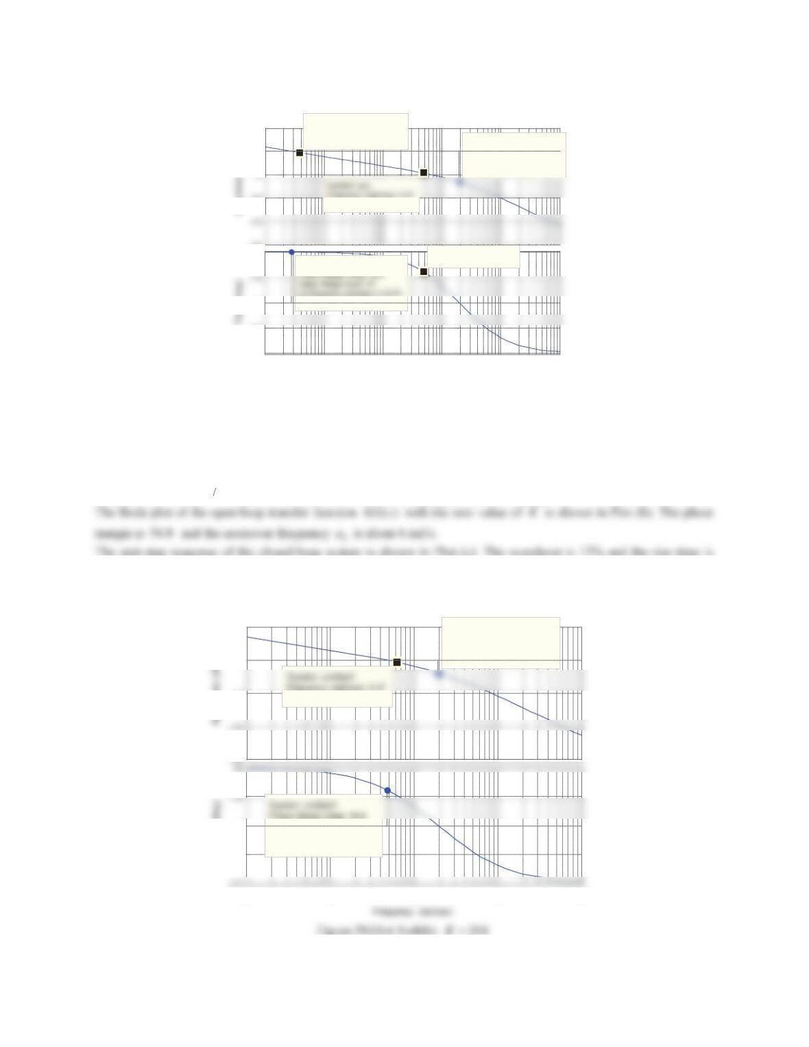
7. Consider the unity negative feedback system shown in Figure 10.77.
a. Use MATLAB to obtain the Bode plot KG(s) for K= 2.
b. Determine the stability of the closed-loop system when K= 2 using the stability margins.
c. Determine the value of Kthat would yield a PM of 30q.
d. Verify the result obtained in Part (c) by using the MATLAB command margin.
Figure 10.77 Problem 7.
Solution
a. The Bode plot of
()KG s
when
2K
is shown in the figure below. The following is the MATLAB session.
>> num = 40*[1 20]; den = conv([1 3 0],[1 10]);
467
Bode Diagram
Frequency (rad/sec)
10
-1
10
0
10
1
10
2
10
3
-225
-135
-90
Delay Margin (sec): 0.571
At frequency (rad/sec): 10.9
Closed Loop Stable? No
System: untitled1
-50
50
100
System: untitled1
Gain Margin (dB): –3.14
At frequency (rad/sec): 9.26
Closed Loop Stable? No
Figure PS10-6 No7
c. To yield a phase margin of
30
D
, the phase when the magnitude plot crosses 0 dB should be
150
D
. It is
observed from the Bode plot of
()KG s
with
2K
that the frequency corresponding to
150
D
is 3.6 rad/s, at
which the magnitude is 19.1 dB. To make the magnitude be 0 dB, the magnitude plot should slide downward by
19.1 20
10 9.02
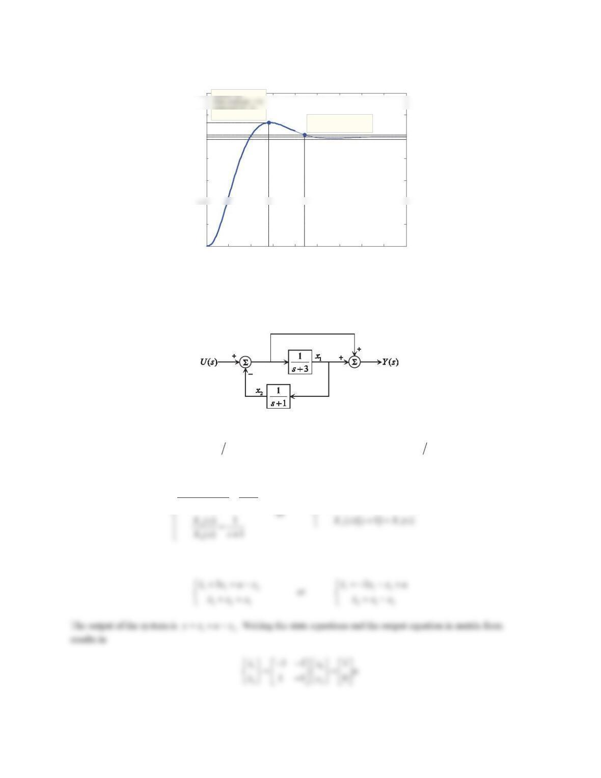
8. Reconsider the feedback system in Figure 10.62. Using the Bode plot technique, find a value of Ksuch that
the maximum overshoot in the response to a unit-step reference input is less than 20% and the 2% settling time
is less than 1.1 s. Plot the unit-step response of the closed-loop system to verify the result.
Solution
The open-loop transfer function is
10 5.5
() 40 5 10
s
KG s K ss s s
468
Bode Diagram
Frequency (rad/sec)
10-2 10-1 100101102103
-270
-225
-180
-90
System: sys
Closed Loop Stable? Yes
Frequency (rad/sec): 4.8
Phase (deg): -125
-200
-100
0
50
System: sys
Gain Margin (dB): 65.4
At frequency (rad/sec): 19.4
Closed Loop Stable? Yes
System: sys
Frequency (rad/sec): 0.0388
Magnitude (dB): -3
Magnitude (dB): –46.2
Figure PS10-6 No8a: K= 1
In order to meet both requirements, we must adjust the value of the proportional control gain
K
. Let us pick
PM 55 D
. This implies that the phase when the magnitude plot crosses 0 dB should be
125D
. It is observed from
the figure above that the frequency corresponding to
125
D
is 4.8 rad/s, at which the magnitude is 46.2dB. To
make the magnitude be 0 dB, the magnitude plot should slide upward by 46.2 dB. This is the effect of multiplying a
constant term of
46.2 20
10 204.17
, which is the value of the proportional control gain
K
.Let us set
K
to be 204.
0.884 s. Both requirements are met.
Bode Diagram
10
-1
10
0
10
1
10
2
10
3
-225
-180
Delay Margin (sec): 0.199
At frequency (rad/sec): 4.81
Closed Loop Stable? Yes
Phase (deg)
-50
0
50 System: untitled1
Gain Margin (dB): 19.3
At frequency (rad/sec): 19.4
Closed Loop Stable? Yes
Magnitude (dB): -3.01
469
Step Response
Time (sec)
Amplitude
00.2 0.4 0.6 0.8 11.2 1.4 1.6 1.8
0
0.2
0.6
0.8
1
1.2
At time (sec): 0.561
System: clp
Settling Time (sec): 0.884
Figure PS10-6 No8(c)
Problem Set 10.7
1. For the system shown in Figure 10.79, derive the state-space equations using the state variables indicated. Make
sure to give the A,B,C,and Dmatrices. Solve for the poles of the system.
Figure 10.79 Problem 1.
Solution
Note that the input to the subsystem
13s
is
2
ux
and the input to the subsystem
11sis
1
x
. The outputs
of these two subsystems are defined as the states
1
x
and 2
x. Thus, in the Laplace domain, we have
1
2
() 1
() () 3
Xs
Us X s s
°
°
12
() 3 () ()
Xss Us Xs
Taking the inverse Laplace transform gives
470
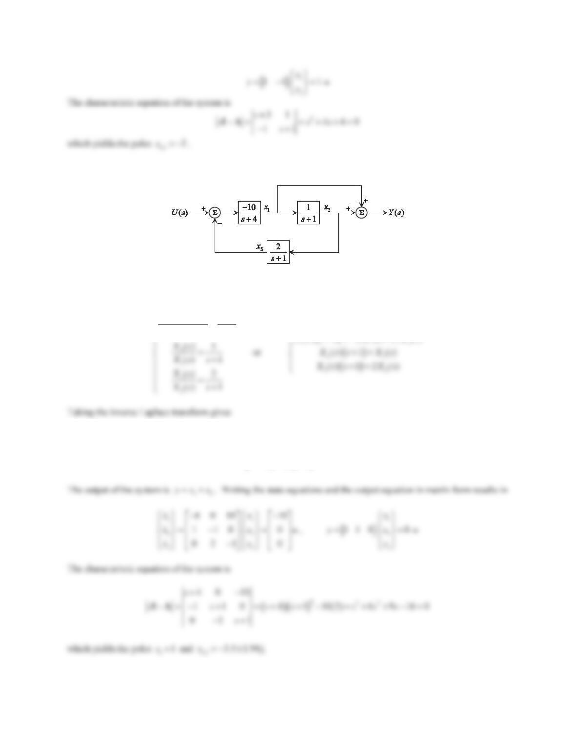
2. Repeat Problem 1 for the system shown in Figure 10.80.
Figure 10.80 Problem 2.
Solution
In the Laplace domain, we have
1
3
() 10
() () 4
Xs
Us X s s
°
°
() 4 10 () 10 ()
Xss Us Xs
113
212
323
41010
2
xxxu
xxx
xxx
°
®
°
¯
3. Determine the controllability and observability for each of the following systems.
a.
>@
11 1
22 2
33 3
530 2
200 0, 016
010 0
xx x
xxuyx
xx x
½ ½ ½
ªºªº
°° °° °°
«»«»
®¾ ®¾ ®¾
«»«»
°° °° °°
«»«»
¬¼¬¼
¯¯ ¯
¿¿ ¿
b.
>@
11 1
22 2
33 3
112 2
400 0, 221
002 0
xx x
xxuyx
xx x
½ ½ ½
ªºªº
°° °° °°
«»«»
®¾ ®¾ ®¾
«»«»
°° °° °°
«»«»
¬¼¬¼
¯¯ ¯
¿¿ ¿
c.
>@
11 1
22 2
33 3
10 0 1
020 1, 110
07 6 1
xx x
xxuyx
xx x
½ ½ ½
ªºªº
°° °° °°
«»«»
®¾ ®¾ ®¾
«»«»
°° °° °°
«»«»
¬¼¬¼
¯¯ ¯
¿¿ ¿
d.
>@
11 1
22 2
33 3
100 0
0 1 0 0 , 111
043 1
xx x
xxuyx
xx x
½ ½ ½
ªºªº
°° °° °°
«»«»
®¾ ®¾ ®¾
«»«»
°° °° °°
«»«»
¬¼¬¼
¯¯ ¯
¿¿ ¿
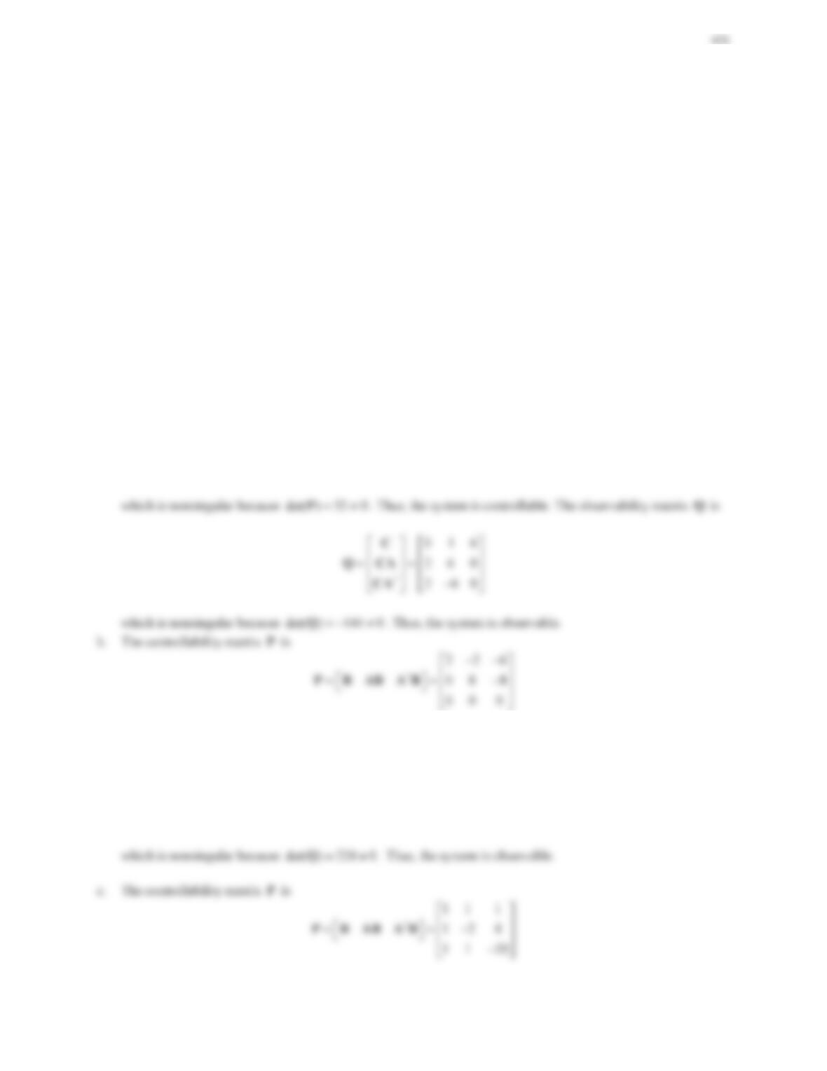
Solution
a. The controllability matrix
P
is
2
21038
04 20
00 4
ªº
«»
ªº
¬¼
«»
«»
¬¼
PBABAB
which is singular. Thus, the system is uncontrollable. The observability matrix
Q
is
2
221
622
14 6 16
ªºª º
«»« »
«»« »
«»« »
¬¼¬ ¼
C
QCA
CA
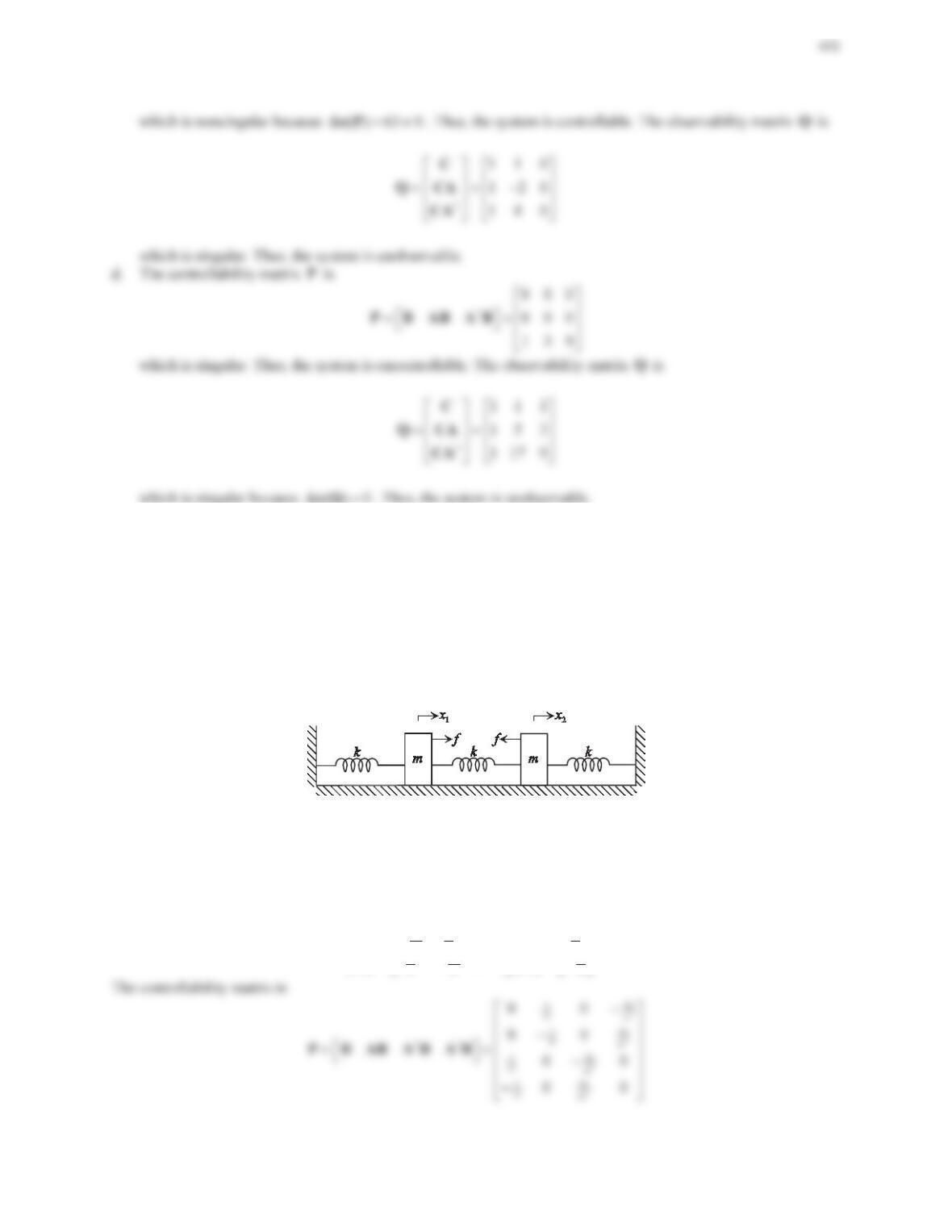
4. Consider the two-degree-of-freedom mass–spring system as shown in Figure 10.81, where two masses are to be
controlled by two equal and opposite forces f. The equations of motion of the system are given by
112
21 2
2,
2.
mx kx kx f
mx kx kx f
Show that the system is uncontrollable. Using the concept of mode discussed in Section 9.4, associate a physical
meaning with the controllable and uncontrollable modes.
Figure 10.81 Problem 4.
Solution
Choosing the state vector
>@
1212
T
xxxx x
and writing the equations of motion in the state-space form
11
22
21
11
21
22
0010 0
0001 0
00
00
kk
mm m
kk
mm m
xx
xx
f
xx
xx
ªºªº
½ ½
«»«»
°° °°
°° °°
«»«»
®¾ ®¾
«»«»
°° °°
«»«»
°° °°
¯¿ ¯¿
¬¼¬¼
473
which is not full rank because the first two rows are dependent with each other and it is same for the last two rows.
Thus, the system is uncontrollable. If we rewrite the equations of motion in the second-order form
11
22
02
02
xx
mkkf
xx
mkk f
½ ½½
ªº ª º
®¾ ®¾® ¾
«» « »
¯¿
¬ ¼¯¿¬ ¼¯¿
5. Reconsider Example 10.22. Using the approach in Section 4.4.1, find the controllable canonical form for the
plant transfer function and then design a full-state feedback controller that places the closed-loop poles at the
same locations as in the example.
Solution
The transfer function of the plant is given by
2
( ) 3.778
() ( ) 16.883
Ys
Gs Us s s
6. A regulation system has a plant with the transfer function
32
() 2
() .
() 2510
Ys
Gs Us sss
a. Transform the plant transfer function into the state-space form with the state vector
[]
T
yyy x
.
b. Determine the state-feedback gain matrix Ksuch that the closed-loop poles are located at p1,2 =í3 ± 3j and
p3=í5.
c. Verify the result in Part (b) by using the MATLAB command place.
Solution
a. Choose the state vector as
>@
T
yyy x
. The transfer function can be converted to the state-space form
010 0
001 0
10 5 2 2
u
ªºªº
«»«»
«»«»
«»«»
¬¼¬¼
xx
,
>@
100y x
c. The following is the MATLAB session used to compute a full-state feedback control gain matrix
K
using
pole placement design.
475
7. Consider the system
>@
11 1
22 2
01 0
,10.
52 1
xx x
uy
xx x
½ ½ ½
ªºªº
®¾ ®¾ ®¾
«»«»
¯¿ ¯¿ ¯¿
¬¼¬¼
a. Design a state-feedback controller so that the closed-loop poles have a damping ratio ȗ and a natural
IUHTXHQF\Ȧn= 5 rad/s.
b. Verify the result in Part (a) by using the MATLAB command place.
Solution
a. For a second-order single-input-single-output system, the gain matrix Kis a
12u
matrix and
>@
12
kk K
b. The following is the MATLAB session used to compute a full–state feedback control gain matrix
K
using
pole placement design.
>> A = [0 1; -5 -2];
8. Consider the system
() 1
() .
()(2)(3)(4)
Ys
Gs Us s s s
476
a. Design a state-feedback controller so that the closed-loop response has an overshoot of less than 5% and a
rise time under 0.5 s. Set one of the closed-loop poles at í10.
b. Verify the result in Part (a) by using the MATLAB command place.
Solution
a. For the plant
32
() 1 1
() ( ) 2 3 4 9 26 24
Ys
Gs Us s s s s s s
And the third one is given, 310p . Thus, the desired characteristic equation of the closed-loop system is
32
3.75 3.31j 3.75 3.31j 10 17.5 100 250 0ssssss
477
Problem Set 10.8
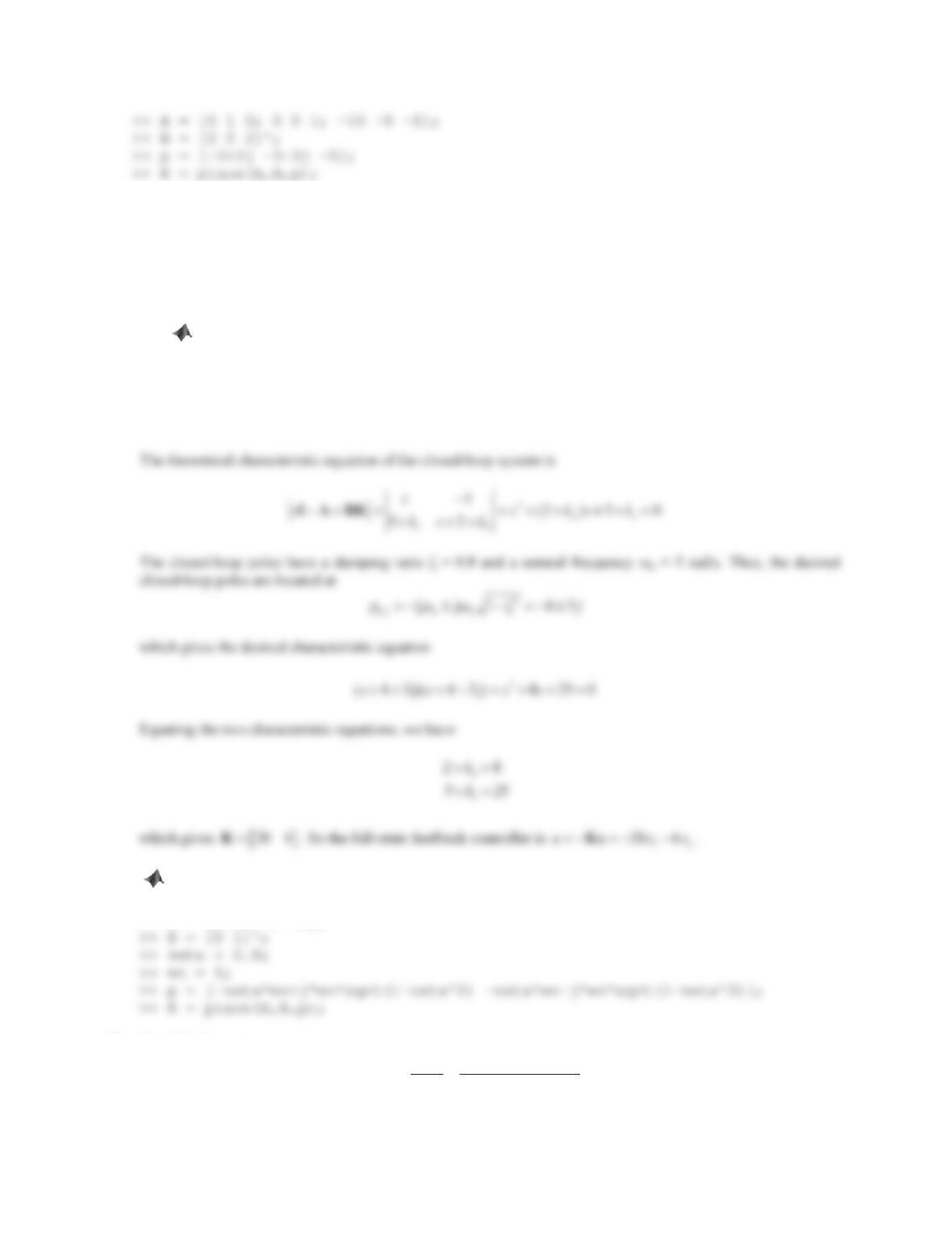
1. Consider the control system shown in Figure 10.40 (Problem Set 10.4, Problem 3). Using the results
obtained in Part (a), build a Simulink block diagram to simulate the feedback control system and find the unit-
step response of the closed-loop system.
Solution
2.25
kp
8
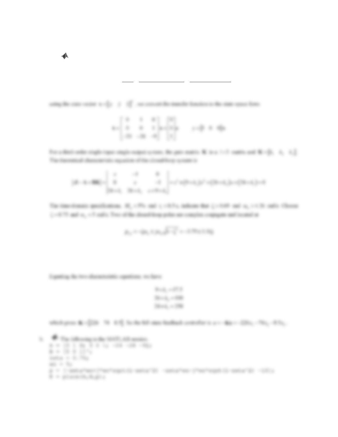
2. Repeat Problem 1 for the control system shown in Figure 10.41 (Problem Set 10.4, Problem 4).
Solution
1
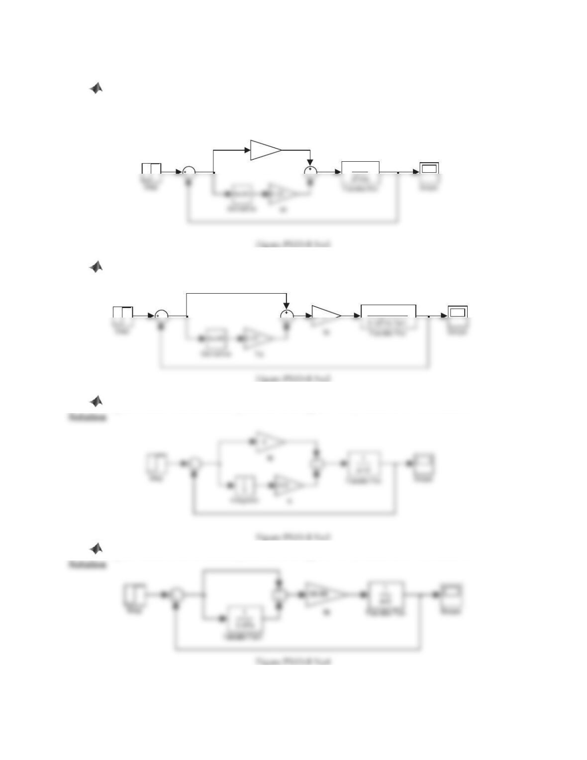
3. Repeat Problem 1 for the control system shown in Figure 10.42 (Problem Set 10.4, Problem 5).
4. Repeat Problem 1 for the control system shown in Figure 10.43 (Problem Set 10.4, Problem 6).
5. Consider the control system shown in Figure 10.61 (Problem Set 10.5, Problem 6). Using the results
obtained in Part (b), build a Simulink block diagram to simulate the feedback control system and find the unit-
step response of the closed-loop system.
6. Repeat Problem 5 for the control system shown in Figure 10.62 (Problem Set 10.5, Problem 7).
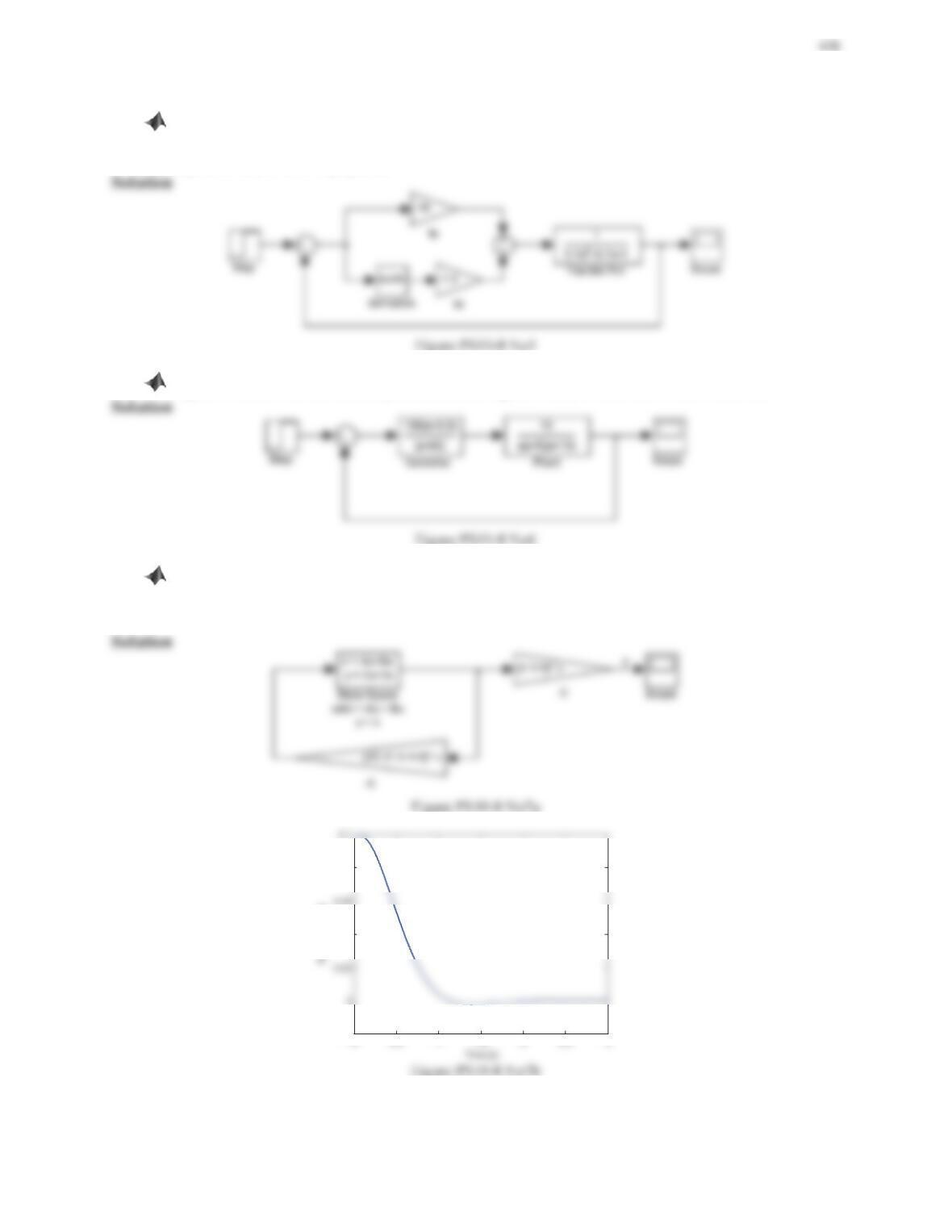
7. Consider Problem 6 in Problem Set 10.7. Using the state-space model obtained in Part (a) and the full-state
feedback controller obtained in Part (b), build a Simulink block diagram to simulate the resulting feedback
control system. Find the closed-loop response if the initial conditions are y(0) = 0.1,
(0) 0y
, and
(0) 0y
.
-0.02
0.04
0.08