Unlock document.
This document is partially blurred.
Unlock all pages and 1 million more documents.
Get Access
379
Problem Set 9.1
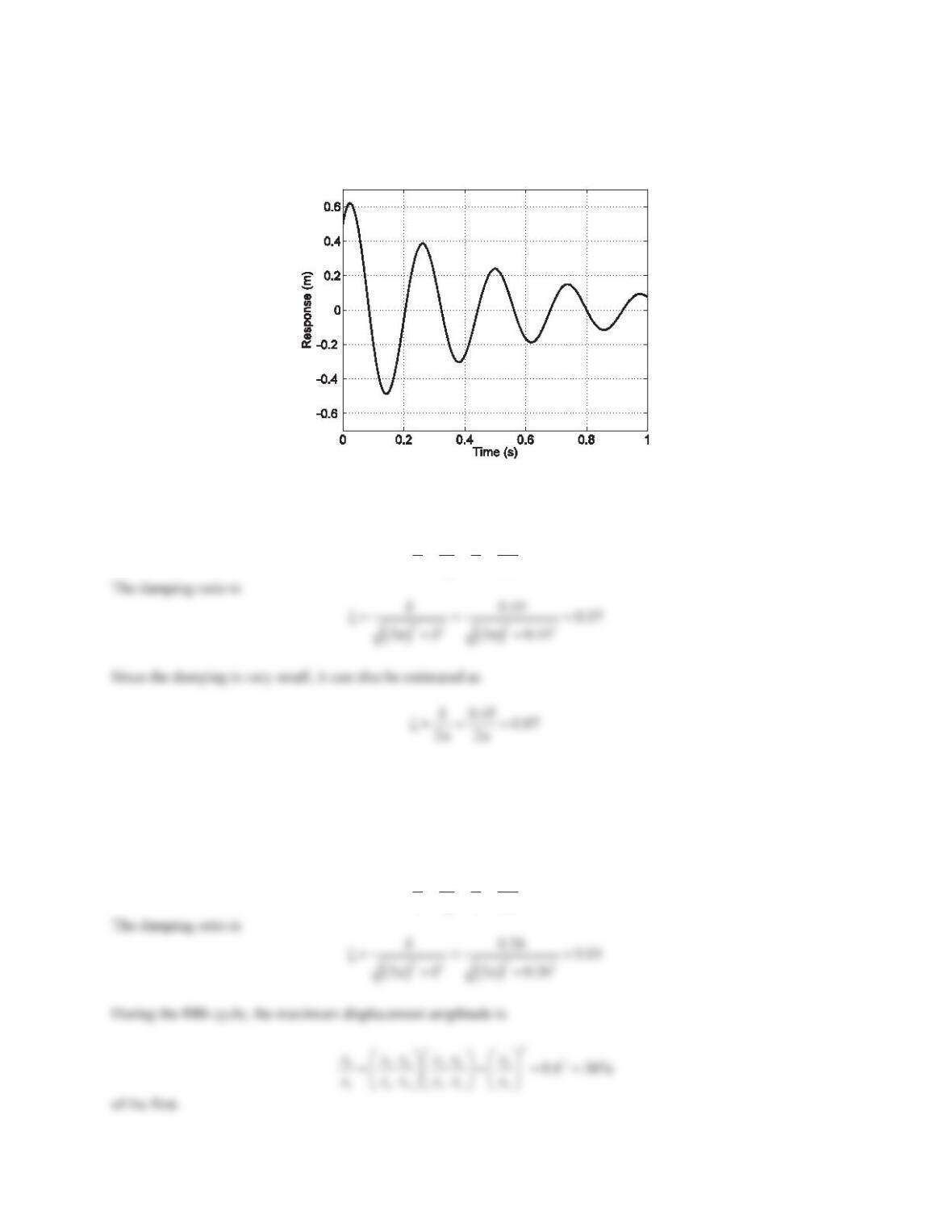
1. A lightly damped single-degree-of-freedom system is subjected to free vibration. The response of the system is
shown in Figure (VWLPDWHWKHYDOXHRIWKHYLVFRXVGDPSLQJUDWLRȗ.
Figure 9.5 Problem 1.
Solution
Note that the first and fifth peak displacements are about 0.62 m and 0.09 m, respectively. Thus, the logarithmic
decrement is
1
5
1 1 0.6
į OQ OQ
4 4 0.1
x
x
2. An underdamped single-degree-of-freedom vibrating system is viscously damped. It is observed that the
maximum displacement amplitude during the third cycle is 60% of the fLUVW&DOFXODWHWKHGDPSLQJUDWLRȗDQG
determine the maximum displacement amplitude during the fifth cycle as a fraction of the first.
Solution
It is observed that the maximum displacement amplitude during the third cycle is 60% of the first. Thus, the
logarithmic decrement is
1
3
111
į OQ OQ
2 2 0.6
x
x
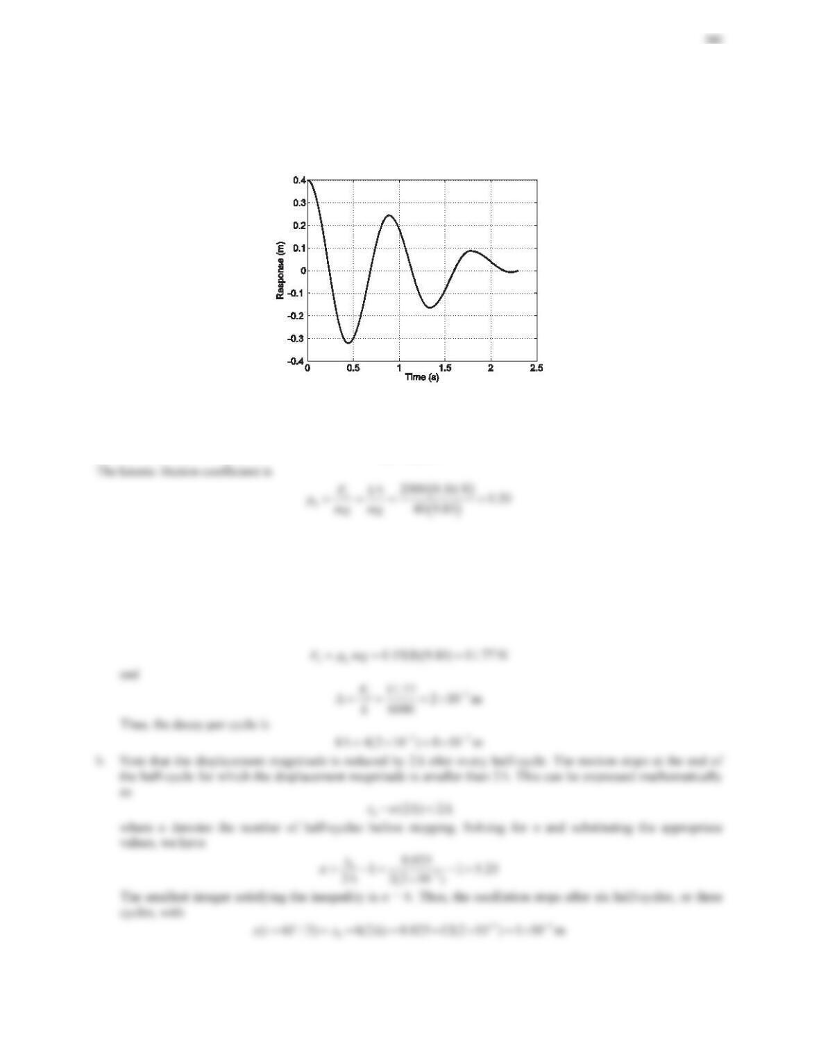
3. Figure 9.6 is the free response of a single-degree-of-freedom system subjected to Coulomb damping. The
parameters of the system include the mass, m= 40 kg, and the spring stiffness, k= 2000 N/m. Estimate the
value of the kinetic friction coefficient ȝk.
Figure 9.6 Problem 3.
Solution
Note that the first, second, and third peak displacements are about 0.4 m, 0.24 m, and 0.09 m, respectively. Thus, the
decay per cycle is
4 0.16'
m
4. A Coulomb damped vibrating system consists of a mass of 8 kg and a spring of stiffness 6000 N/m. The kinetic
IULFWLRQFRHIILFLHQWȝkis 0.15. The initial conditions are x0= 0.025m and v0= 0m/s.
a. Determine the decay per cycle.
b. Determine the position when the oscillation stops.
Solution
a. The magnitude of the Coulomb damping force is
381
Problem Set 9.2
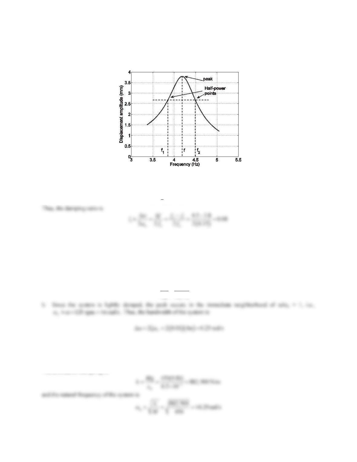
1. Figure 9.13 shows the experimental data for the frequency response of a single-degree-of-freedom system. Use
the half-power bandwidth method to eVWLPDWHWKHGDPSLQJUDWLRȗRIWKHV\VWHP
Figure 9.13 Problem 1.
Solution
Note that the frequencies corresponding to half-power points, f1and f2, are about 3.8 Hz and 4.5 Hz, respectively.
For light damping, the natural frequency is
1
n12
2
4.15fff|
Hz
2. A viscously damped single-degree-of-freedom system is subjected to a harmonic force excitation. It is observed
that the amplitude of the frequency response X/xst reaches the maximum when the driving frequency is 120 rpm.
The peak value is 50. Assume the system to be lightly damped.
a. 'HWHUPLQHWKHGDPSLQJUDWLRȗ.
b. Determine the bandwidth of the system.
Solution
a. For small damping, the damping ratio can be estimated using the peak amplitude of the frequency response, i.e.,
11
ȗ
2250Q
|
3. An industrial machine of mass M= 450 kg is supported by a spring with a static deflection xst = 0.5 cm. If the
machine has a rotating unbalance me = 0.25 kg·m, determine the dynamic amplitude Xat 1200 rpm. Assume
damping to be negligible.
Solution
The stiffness of the spring is
382
Given the driving frequency of 1200 rpm, the frequency ratio is
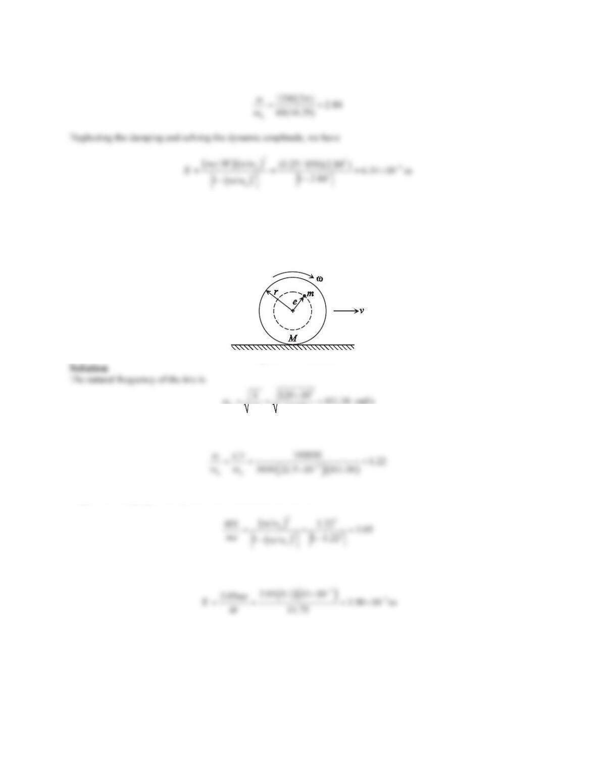
4. Tires must be balanced so that no periodic forces develop during operation. Figure 9.14 shows a tire with an
eccentric mass because of uneven wear. The parameters are given as follows: the mass of the tire M= 11.75 kg,
the unbalanced mass m= 0.1 kg, the radius of the tire r= 22.5 cm, and the eccentric distance e= 15 cm.
Assume that the stiffness of the tire is 120 kN/m. Neglect the damping of the system. Determine the amplitude
of the steady-state response of the tire caused by mass unbalance when the car moves at 100 km/h.
Figure 9.14 Problem 4.
n
11.75
M
When the car moves at 100 km/h, the frequency ratio is
Neglect the damping of the system. The dimensionless ratio is
which gives the amplitude of the steady-state response of the tire as
5. Reconsider Example 9.5, where the mathematical model of a vehicle is given by an ordinary differential
equation mx bx kx bz kz
with m= 3000 kg, b= 2000 Ns/m, and k= 50 kN/m. It is observed that the
base excitation due to the roughness of the road surface is also related to the speed of the vehicle, i.e., z =
0.01sin(0.2Svt). Determine the transmissibility and the dynamic amplitude Xof the vehicle when it moves at a
speed of (a) 25 km/h and (b) 105 km/h.
383
Solution
a. The natural frequency and the damping ratio of the vehicle system are
3
n
50 10
Ȧ
3000
k
m
u
rad/s
When the vehicle moves at a speed of 25 km/h, the frequency of the harmonic excitation is
Thus, the transmissibility is
Thus, the dynamic amplitude of the vehicle is
2
4.52 10X
u
m.
b. When the vehicle moves at a speed of 105 km/h, the frequency of the harmonic excitation is
and the frequency ratio is n
Ȧ Ȧ
. Thus, the transmissibility is
6. Precision instruments must be placed on rubber mounts, which act as springs and dampers, to reduce the effects
of base vibration. Consider a precision instrument of mass 110 kg mounted on a rubber block. For the entire
assembly, the spring stiffness is 280 kN/m and the damping ratio is 0.10. Assume that the base undergoes
vibration, and the displacement of the base is expressed as y(t) = Y0sin(Ȧt). Determine the dynamic amplitude of
the system if the acceleration amplitude of the base excitation is 0.15 m/s2and the excitation frequency is 20Hz.
Solution
The expression for the acceleration of the base is
2
0
() ȦVLQȦyt Y t
ZKHUH Ȧ2Y0= 0.15m/s2. For an excitation
frequency of 20 Hz, the displacement amplitude of the base is
n
2.49
Ȧ280000 /110
and the transmissibility is
Problem Set 9.3
1. A 90-kg instrument is hung from a ceiling by four springs, each of which has a stiffness of 4 kN/m. The ceiling
vibrates with a frequency of 2 Hz and an amplitude of 0.05 mm due to the air conditioning compressor and
chiller mounted on the roof. Neglecting the damping, determine the maximum displacement amplitude of the
instrument.
Solution
The natural frequency of the instrument is
3
n
4(4 10 )
Ȧ
90
k
m
u
rad/s. When the ceiling vibrates with a
frequency of 2 Hz, the frequency ratio is
2. Consider a 12-kg instrument placed on a floor that vibrates with a frequency of 3500 rpm and an amplitude of 2
mm due to nearby machinery. A vibration isolator is designed to protect the instrument from the vibration of the
floor. Assume that the damping ratio of the isolator is 0.05 and the maximum allowable acceleration amplitude
of the instrument is 2g.
a. Determine the stiffness of the isolator.
b. Determine the maximum displacement amplitude of the instrument.
Solution
a. Assume that the expression for the displacement of the instrument is x(t) = Xsin(Zt+I). The acceleration
amplitude of the instrument is
2
ȦAX
, where the maximum allowable acceleration amplitude is 2g. When the
floor vibrates with a frequency of 3500 rpm and an amplitude of 2 mm, the transmissibility is
Assume that the damping ratio of the isolator is 0.05. The transmissibility can be given by
385
which is equivalent to
3. A 9000-kg air conditioning compressor mounted on a roof is supported by four springs. The static deformation
of each spring is 8 cm. Neglecting the damping, determine the force transmissibility when the compressor
works at 60 Hz.
Solution
The equivalent spring stiffness is
eq
9000(9.81) 1103.63
0.08
mg
k
'
kN. Thus, the natural frequency of the system is
4. Consider the single-degree-of-freedom system shown in Figure 9.8. The excitation force due to the rotating
unbalance is meȦ2sin(Ȧt). Assume that the system has the following parameters: m= 5 kg, M= 100 kg, e= 0.1
m, k= 5000 N/m, and b= 200 N·s/m.
a. 'HWHUPLQHWKHIRUFHWUDQVPLWWHGWRWKHVXSSRUWZKHQWKHV\VWHPUXQVDWWKHURWDWLQJVSHHGȦ Ȧn.
b. Determine the force transmissibility.
c. The spring is replaced in order to decrease the force transmissibility to 20%. Determine the stiffness of the
new spring.
Solution
a. The natural frequency of the system is
n
5000
Ȧ
k
rad/s
386
When the system runs at the rotating speed Ȧ Ȧn, the dimensionless ratio is
Thus, the dynamic amplitude is
100
The force transmitted to the support is
b. The force transmissibility is
c. If the force transmissibility is decreased to 20%, solving for
2
n
ȦȦ
gives
2
n
Ȧ Ȧ
,with the
negative value rejected. Thus, the new natural frequency is
5. A rotating machine has a mass of 6 kg and a natural frequency of 5 Hz. Due to a rotating unbalanced mass, the
machine is subjected to a harmonic disturbance force meȦ2sin(Ȧt). When the machine operates at a frequency of
3.5 Hz, the amplitude of the disturbance force is 40 N.
a. Design a vibration absorber assuming that the maximum allowable displacement of the absorber is 5 cm.
b. Using MATLAB, write an m-file to plot X1/me YHUVXVȦ.
Solution
a. The natural frequency of the absorber is required to be the same as the disturbance frequency,
2
Ȧ Ȧ +] ʌ
rad/s
The maximum allowable displacement amplitude of the absorber is 5 cm. Thus, the spring stiffness of the
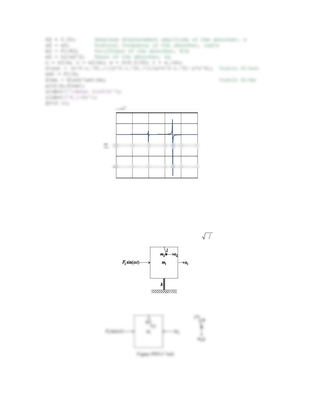
387
010 20 30 40 50
-4
-2
0
1
2x 10
Z
(rad/s)
X
Figure PS9-3 No5
6. The pendulum in Figure 9.19 is known as a tuned mass damper. It is mounted in a building, which is simplified
as a block of mass m1supported by a spring of stiffness k. The mass of the pendulum is m2and the length lis
tunable. The tunable pendulum is used to control the vibration of the building under extreme wind loads.
Assume that the force due to gusty winds can be modeled as a harmonic force F1sin(Zt), and the excitation
frequency Zis very close to the natural frequency of the building. Prove that the forced vibration of the building
can be eliminated when the length of the pendulum is tuned such that Ȧgl , where gis the gravitational
acceleration.
Figure 9.19 Problem 6.
Solution
Assume that x2>x1> 0. The free-body diagram of the building and the pendulum is shown in the figure below.
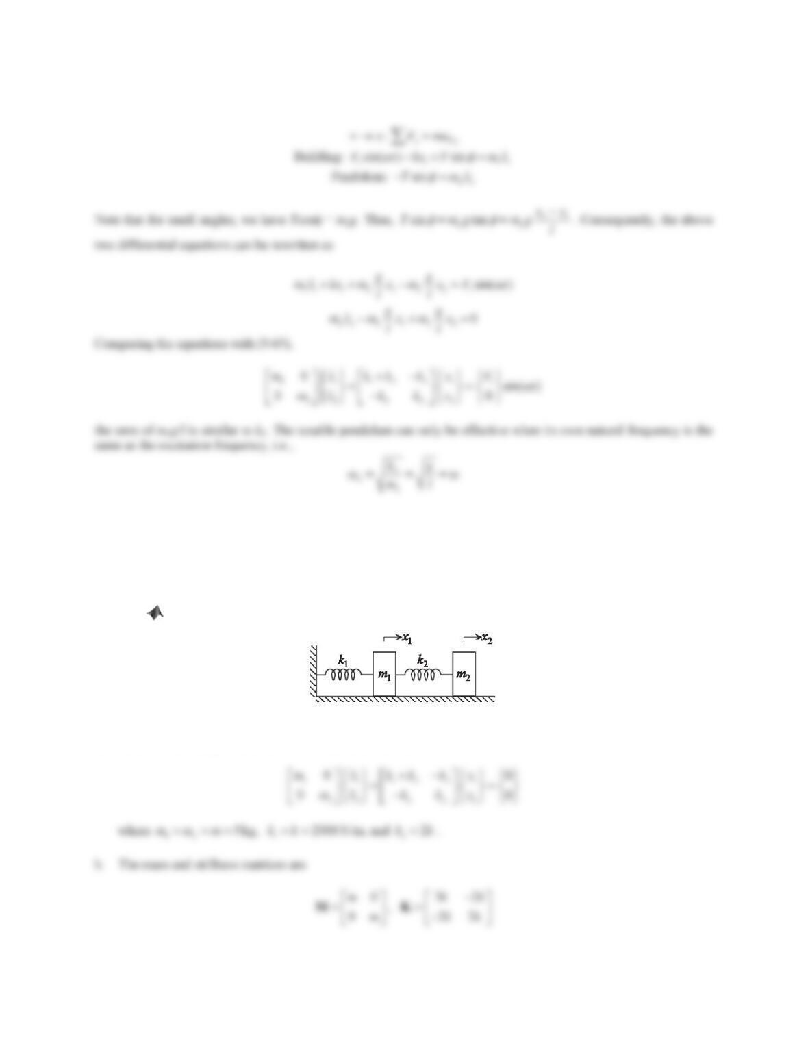
388
Applying Newton’s second law along x-direction gives
Problem Set 9.4
1. Consider the two-degree-of-freedom mass–spring system shown in Figure 9.22. Assume that m1=m2=m,k1=
k, and k2= 2k, where m= 5 kg and k= 2000 N/m.
a. Derive the equations of motion and write them in matrix form.
b. Solve the associated eigenvalue problem by hand. Plot the two modes and explain the nature of the mode
shapes.
c. Solve the associated eigenvalue problem using MATLAB.
Figure 9.22 Problem 1.
Solution
a. The differential equations of motion in matrix form are
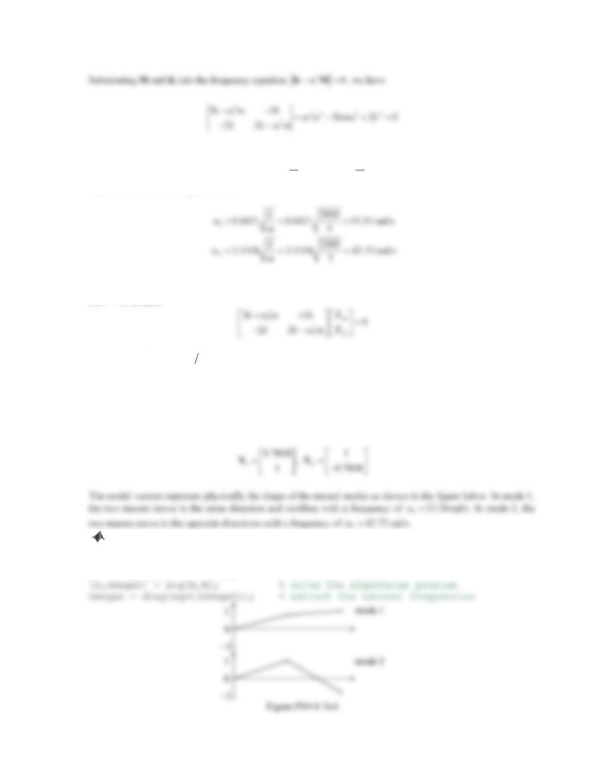
389
which gives the two eigenvalues
2
1
Ȧ k
m
,
2
2
Ȧ k
m
Thus, the two natural frequencies are
To determine the eigenvectors or modal vectors, we insert
2
Ȧ
r
(r= 1, 2) into the equation
2
Ȧ KMX0
.
For r= 1, we have
Substituting
2
1
Ȧ km
and dividing by kresults in
11
12
2.5616 2 0
2 1.5616
X
X
ªº
ªº
«»
«»
¬¼
¬¼
Assuming
12
1X
leads to
11
0.7808X
. In a similar way, we can find the other modal vector.
c. The following is the MATLAB session.
m = 5; k = 2000;
M = diag([m m]); % mass matrix
K = [3*k -2*k; -2*k 2*k]; % stiffness matrix
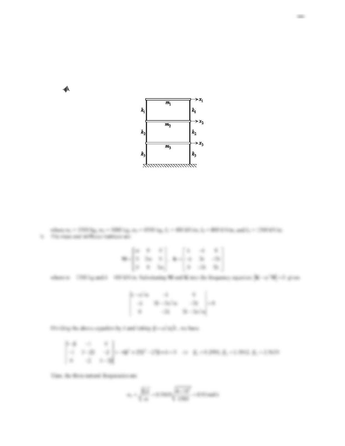
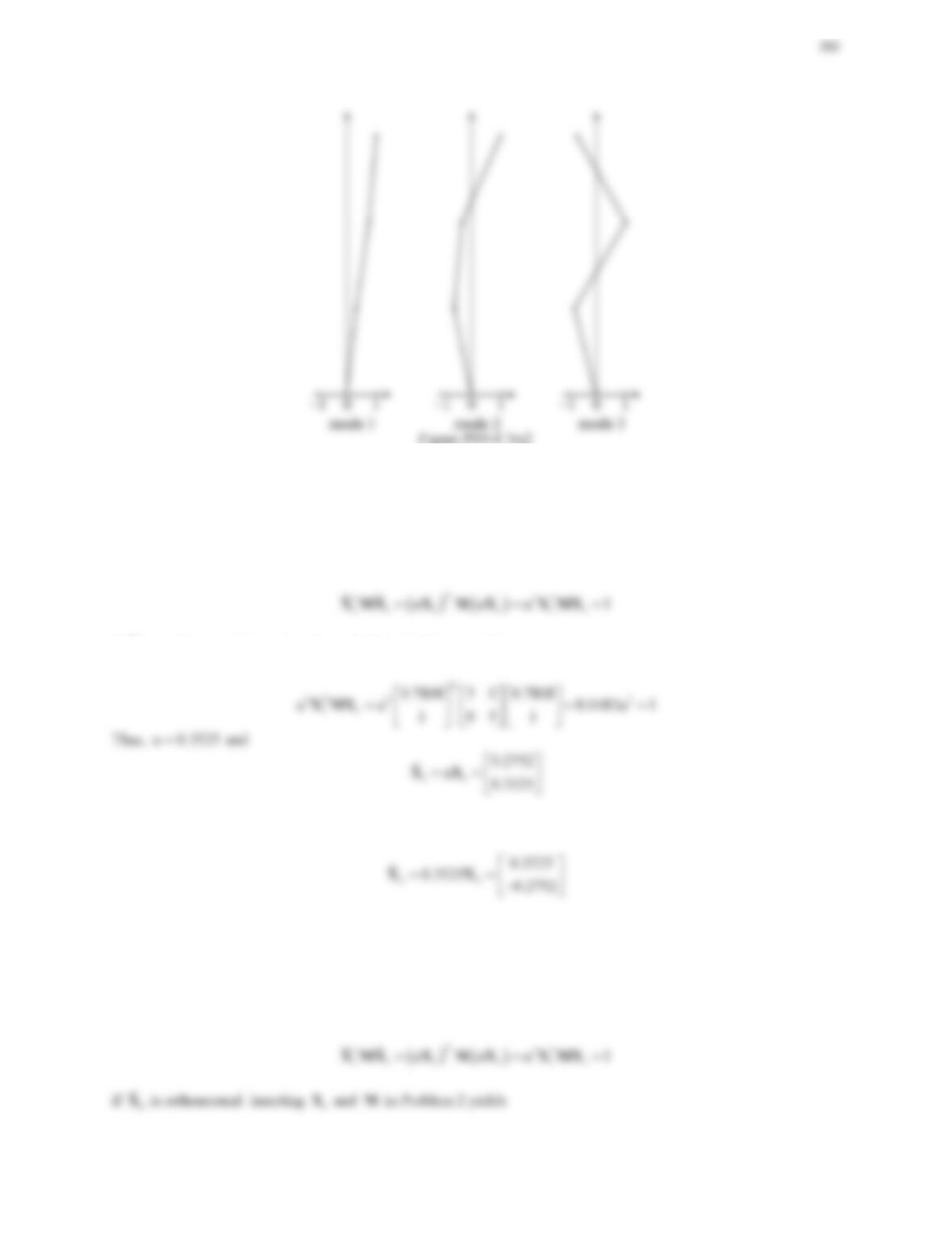
2. A three-story building can be modeled as a three-degree-of-freedom system as shown in Figure 9.23, where the
horizontal members are rigid and the columns are massless beams acting as springs. Assume that m1= 1500 kg,
m2= 3000 kg, m3= 4500 kg, k1= 400 kN/m, k2= 800 kN/m, and k3= 1200 kN/m.
a. Derive the differential equations for the horizontal motion of the masses.
b. Solve the associated eigenvalue problem by hand. Plot the three modes and explain the nature of the mode
shapes.
c. Solve the associated eigenvalue problem using MATLAB.
Figure 9.23 Problem 2.
Solution
a. The differential equations of motion in matrix form are
1111 1
2211222
33 2 233
00 0 0
00 0
00 0 0
mxkkx
mxkkkkx
mx k kkx
½ ½½
ªºª º
°° °°°°
«»« »
®¾ ®¾®¾
«»« »
°° °°°°
«»« »
¯¿
¯¿ ¯¿
¬¼¬ ¼
391
5
2
2
ȕ410
Ȧ
1500
k
m
u
rad/s
5
3
3
ȕ410
Ȧ
1500
k
m
u
rad/s
In a similar way, we can find the other two modal vectors.
2
1
0.3042
ªº
«»
X
3
0.6397
1
ªº
«»
«»
X
c. The following is the MATLAB session.
M = diag([1500 3000 4500]); % mass matrix
K = [400 -400 0; % stiffness matrix
-400 1200 -800;
0 -800 2000]*1000;
3. Consider the two-degree-of-freedom mass–spring system in Figure 9.22. Normalize the modal vectors X1and
X2obtained in Part (b) of Problem 1 to a set of orthonormal modal vectors satisfying Equations 9.96 and 9.97.
Solution
Write the first modal vector in the form
11
Į XX
,where
1
X
is the modal vector after normalization and
Į
is a
nonzero scaling constant. Substituting
1
X
into Eq. (9.96) gives
if
1
X
is orthonormal. Inserting
1
X
and
M
in Problem 1 yields
Following the same procedure yields the other orthonormal modal vector,
4. Consider the three-story building system in Figure 9.23. Normalize the modal vectors X1,X2, and X3obtained
in Part (b) of Problem 2 to a set of orthonormal modal vectors satisfying Equations 9.96 and 9.97.
Solution
Write the first modal vector in the form
11
Į XX
,where
1
X
is the modal vector after normalization and
Į
is a
nonzero scaling constant. Substituting
1
X
into Eq. (9.96) gives
393
Following the same procedure yields the other two orthonormal modal vectors,
0.0177
ªº
0.0082
ªº
5. Consider the two-degree-of-freedom mass–spring system in Figure 9.22. Determine the response of the system
subjected to initial excitations x(0) = [0 0]Tand
>@
Ú
(0) 1 0 T
x
by modal analysis. Note that the natural
frequencies were solved in Problem 1 and the modal vectors were normalized in Problem 3.
Solution
From Problems 1 and 3, we obtained the two natural frequencies
The modal responses are
1
() (0)cos(Ȧ VLQȦ
Ȧ
TT
rr r r r
r
qt t t r XMx XMx
The response of the system to the given initial excitations is
6. Consider the three-story building system in Figure 9.23. Determine the response of the system subjected to
initial excitations x(0) = [0.01 0 0]Tand
>@
(0) 000
T
x
by modal analysis. Note that the natural frequencies
were solved in Problem 2 and the modal vectors were normalized in Problem 4.
394
Solution
From Problems 2 and 4, we obtained the natural frequencies
1
Ȧ rad/s,
2
Ȧ
rad/s, 3
Ȧ rad/s
and the orthonormal modal vectors
1
0.0169
0.0118
ªº
«»
«»
X
,
2
0.0177
0.0054
ªº
«»
X
,
3
0.0082
0.0128
ªº
«»
«»
X
7. Consider the two-degree-of-freedom mass–spring system in Figure 9.22. Determine the response of the system
if a harmonic force F(t) = 2 cos tis applied to mass 2. Note that the natural frequencies were solved in Problem
1 and the modal vectors were normalized in Problem 3.
Solution
The force vector can be written as
000
cos
() 2cos 2 t
Ft t
½ ½½
®¾® ¾®¾
¯¿¯ ¿¯¿
f
395
The response of the system to the given harmonic excitation is
8. Consider the three-story building system in Figure 9.23. Determine the response of the system if a harmonic
force F(t) = 0.15 sin(0.15t) is applied to the top story. Note that the natural frequencies were solved in Problem
2 and the modal vectors were normalized in Problem 4.
Solution
The force vector can be written as
( ) 0.15sin 0.15 0.15
0 0 0 sin 0.15
000
Ft t
t
½ ½½
°°° °°°
®¾® ¾®¾
°°° °°°
¯¿¯ ¿¯¿
f
where
>@
0.15
0.0169 0.0118 0.0058 0
½
°°
®¾
The response of the system to the given harmonic excitation is
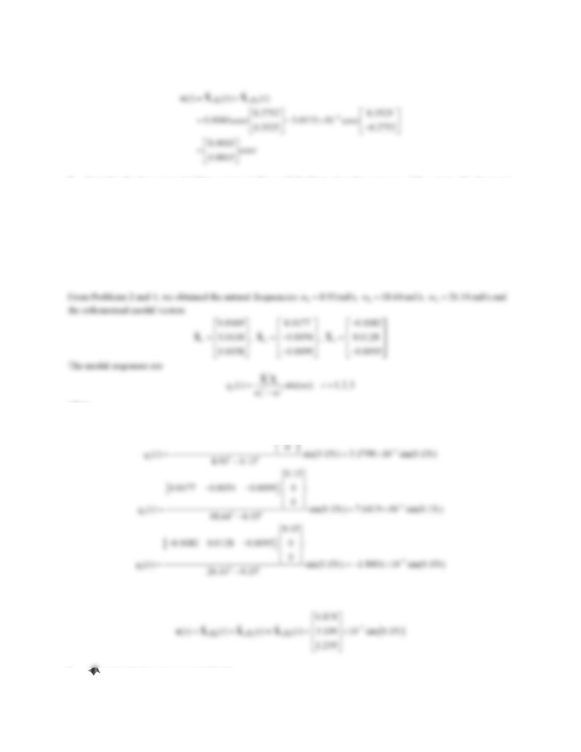
9. Solve Problem 5 using MATLAB.
396
Solution
The following is the MATLAB session written based on Eqs. (9.106) and (9.114).
% eigenvalue problem
m = 5;
k = 2000;
M = diag([m m]); % mass matrix
00.2 0.4 0.6 0.8 1
-0.2
-0.1
0
0.1
0.2
q1
00.2 0.4 0.6 0.8 1
-0.05
0
0.05
q2
Time (s)
00.2 0.4 0.6 0.8 1
-0.05
0
0.05
x1
00.2 0.4 0.6 0.8 1
-0.05
0
0.05
x2
Time (s)
Figure PS9-4 No9a Modal responses. Figure PS9-4 No9b System responses.
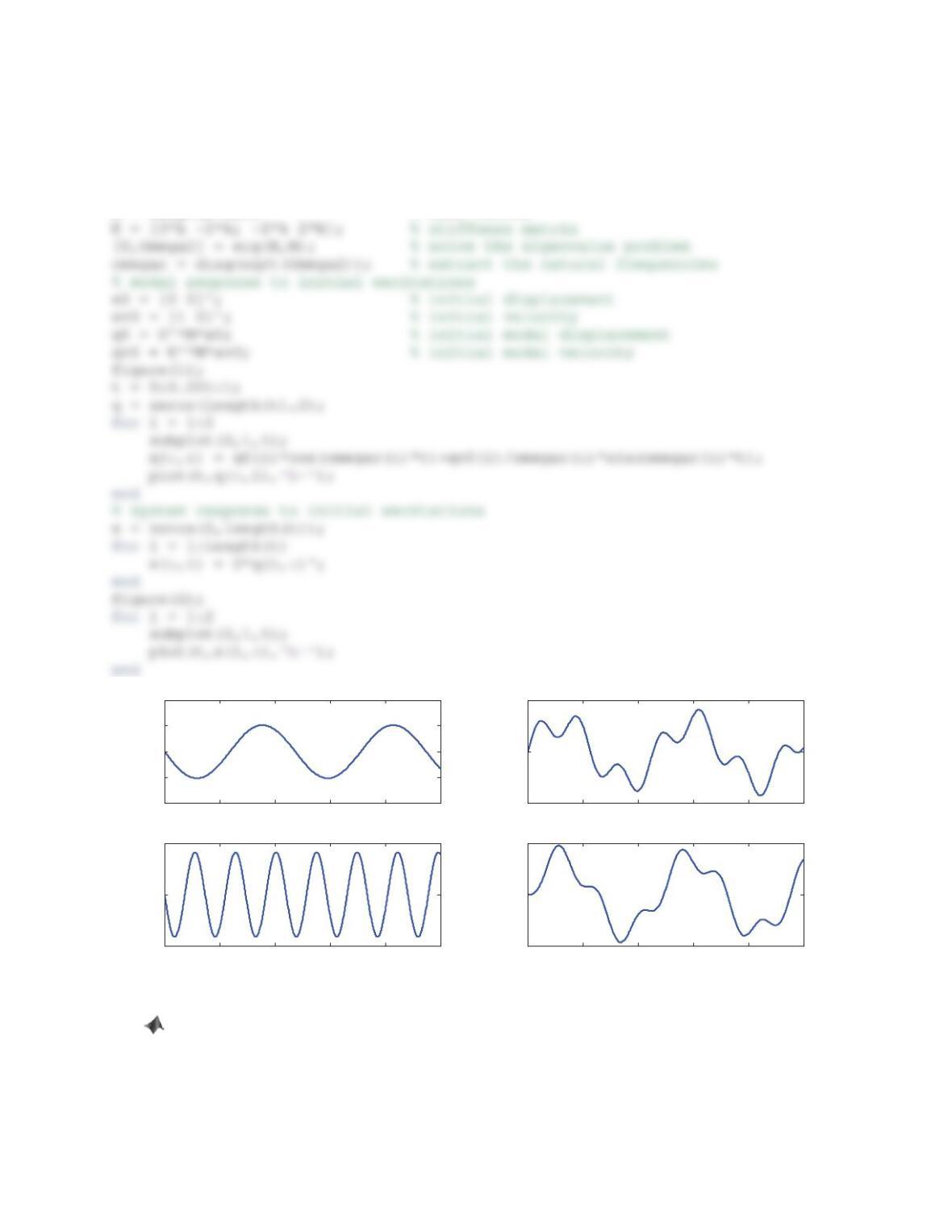
10. Solve Problem 6 using MATLAB.
Solution
The MATLAB session is similar to the one given in Problem 9.
% eigenvalue problem
M = diag([1500 3000 4500]); % mass matrix
-400 1200 -800;
0 -800 2000]*1000;
[U,Omega2] = eig(K,M); % solve the eigenvalue problem
omegar = diag(sqrt(Omega2)); % extract the natural frequencies
% modal response to initial excitations
end
-0.5
0.5
0.5
00.2 0.4 0.6 0.8 1
0.2
Time (s)
-0.01
0.01
x
5x 10
x
00.2 0.4 0.6 0.8 1
0.01
x
Time (s)
Figure PS9-4 No10a Modal responses. Figure PS9-4 No10b System responses.
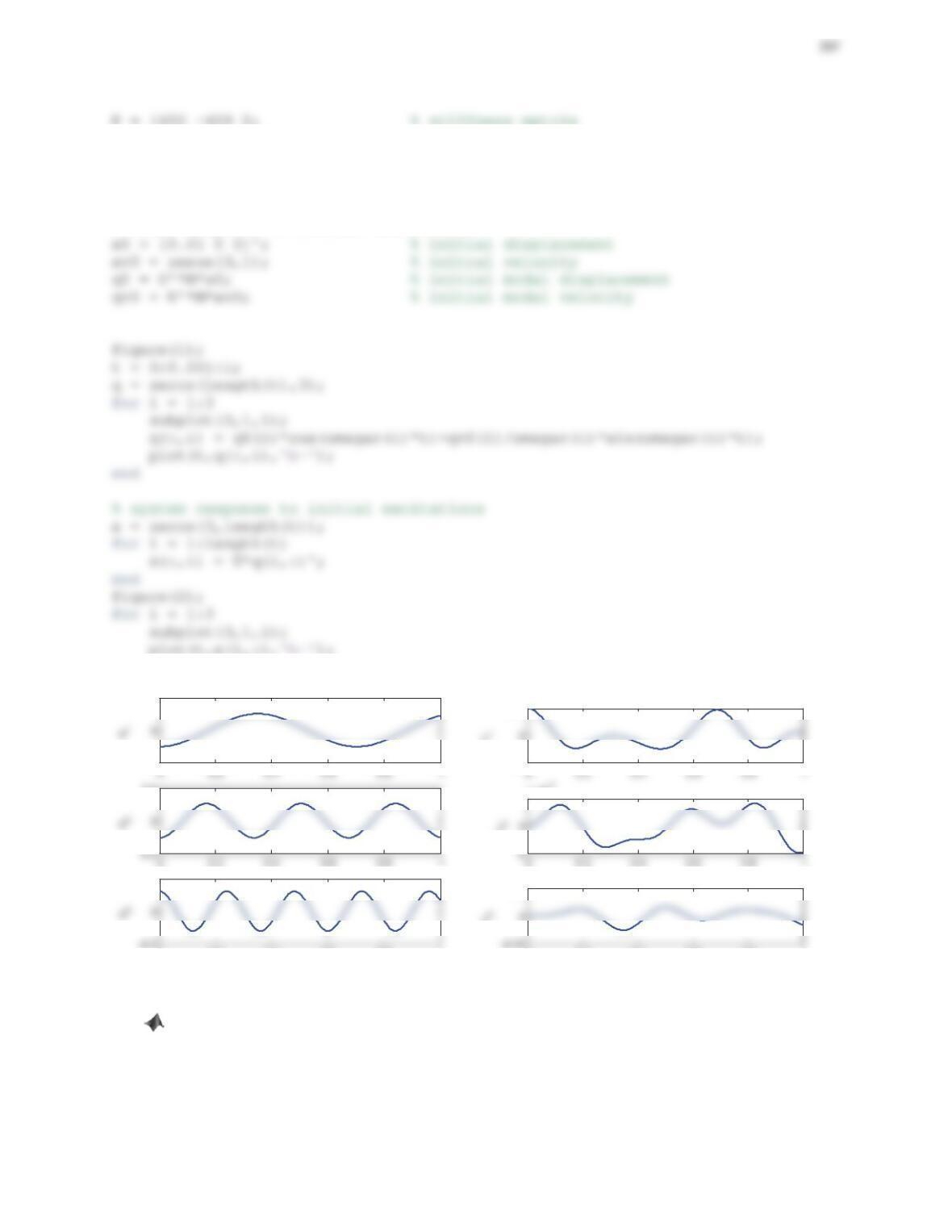
11. Solve Problem 7 using MATLAB.
Solution
The following is the MATLAB session written based on Eqs. (9.121) and (9.122).
% eigenvalue problem
m = 5; k = 2000;
398
% modal response to external excitations
f0 = [0 2]';
for i = 1:2
subplot(2,1,i);
% system response to external excitations
x = zeros(2,length(t));
end
figure(2);
for i = 1:2
subplot(2,1,i);
plot(t,x(i,:),'b-');
end
5x 10
-3
q
0 2 4 6 8 10
-4
-2
4x 10
-4
Time (s)
q
-1
2x 10
-3
x
0 2 4 6 8 10
-2
-1
2x 10
-3
Time (s)
x
Figure PS9-4 No11a Modal responses. Figure PS9-4 No11b System responses.
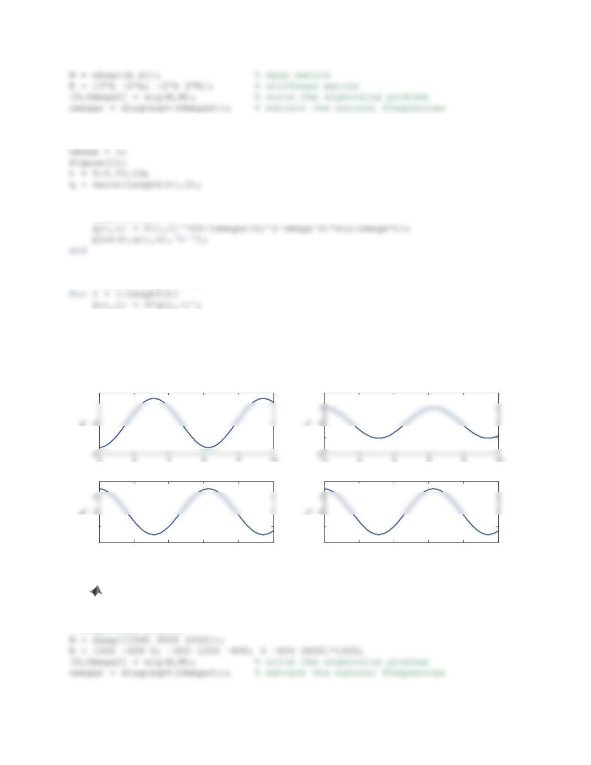
12. Solve Problem 8 using MATLAB.
Solution
The MATLAB session is similar to the one given in Problem 11.
% eigenvalue problem


