439
00.1 0.2 0.3 0.4 0.5 0.6 0.7 0.8
0
0.2
0.6
0.8
1.4
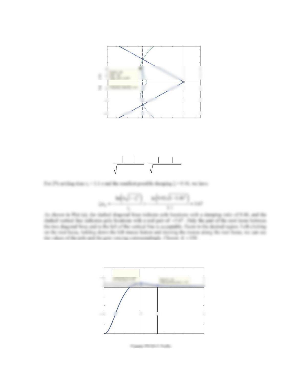
Step Response
Amplitude
Closed-loop response
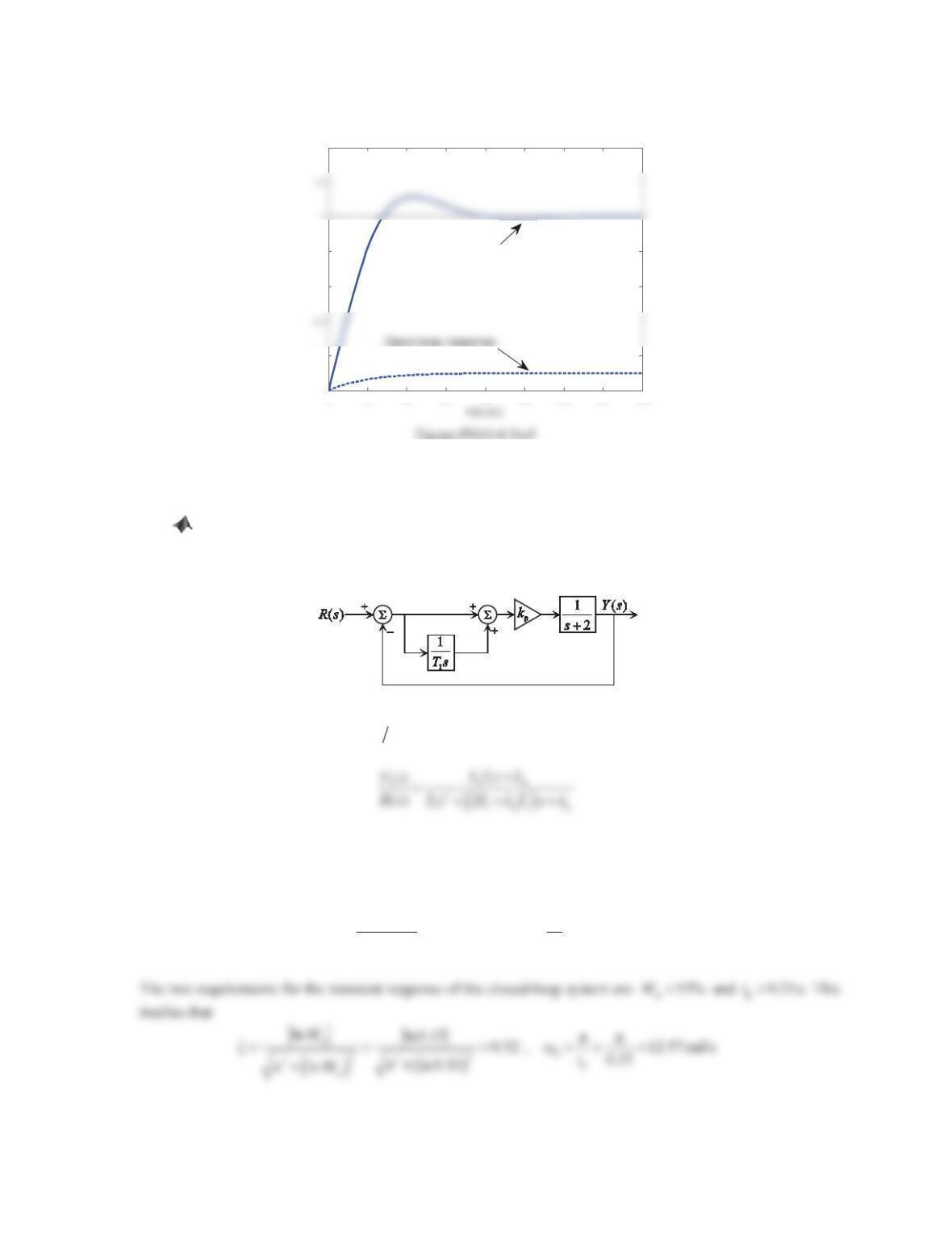
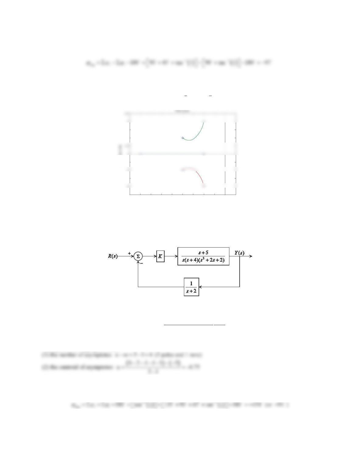
6. Consider the feedback control system shown in Figure 10.43.
a. Find the values for kpand TIsuch that the maximum overshoot in the response to a unit-step reference input
is less than 15% and the peak time is less than 0.25 s.
b. Verify the results in Part (a) using MATLAB by plotting the unit-step response of the closed-loop
system. If the maximum overshoot and the peak time exceed the requirements, make a fine tuning and
reduce them to be approximately the specified values or less.
Figure 10.43 Problem 6.
Solution
a. The closed-loop transfer function () ()Ys Rs is
which is a second-order system. The closed-loop characteristic equation is
2
IIpIp
20Ts T kT s k
.
Denoting the natural frequency and the damping ratio of the closed-loop system as
n
Ȧ
and
ȗ
, we have
IpI p 2
pn n
II
222ȗȦ Ȧ
TkT k
k
TT
440
b. Below is the MATLAB session.
sys = tf([1],[1 2]);
Ti = 0.07;
Step Response
Time (sec)
00.05 0.1 0.15 0.2 0.25 0.3
0.4
1
1.2
1.4 System: clp
Peak amplitude: 1.14
Overshoot (%): 14
At time (sec): 0.0938
Figure PS10-4 No6
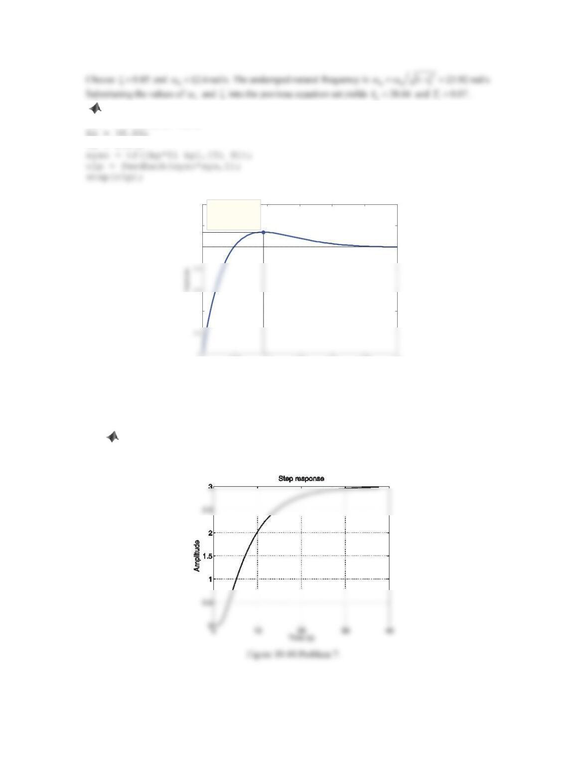
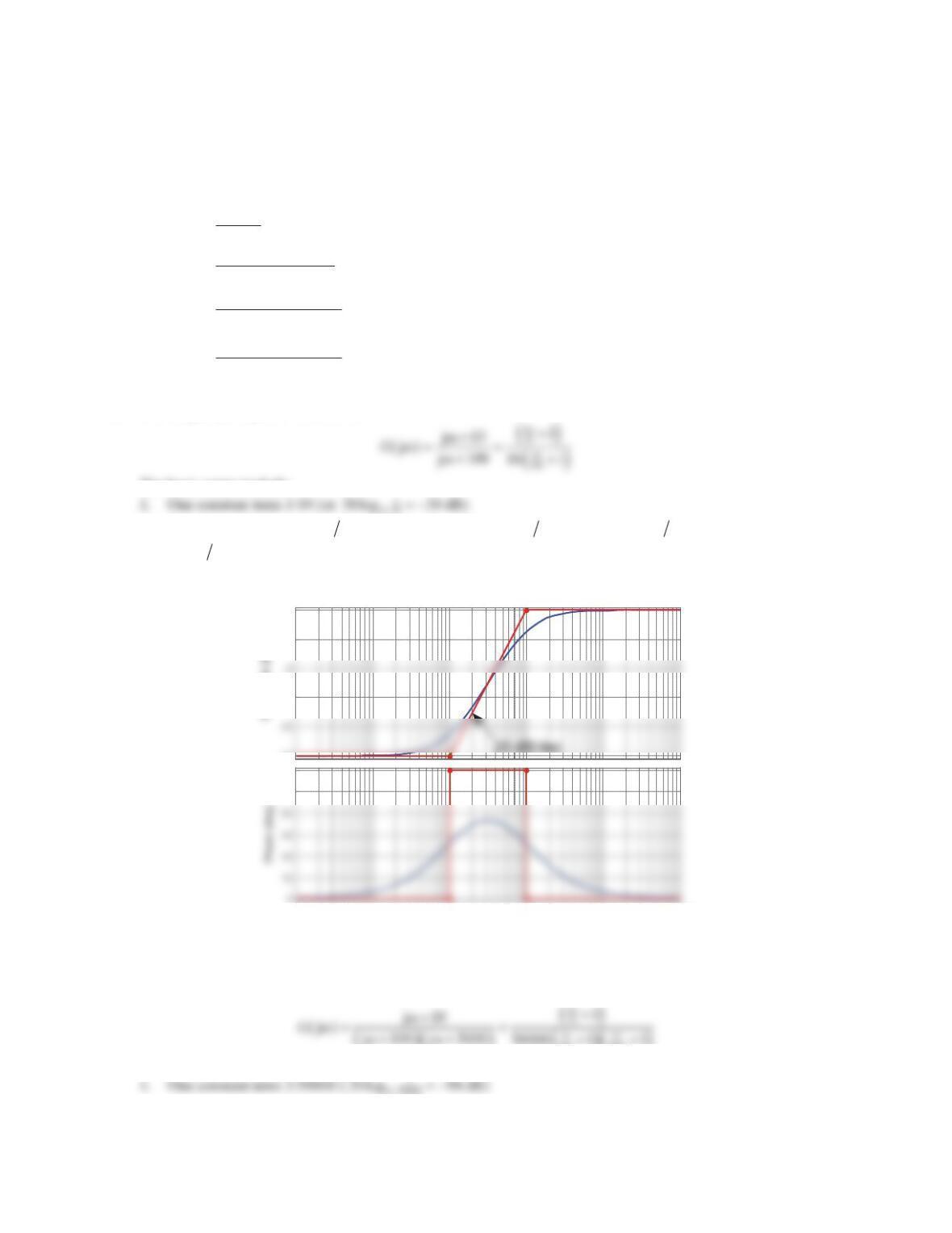
7. The unit-step response of a plant is shown in Figure 10.44.
a. The lag time Land the reaction rate Rcan be determined from the figure. Find the P, PI, and PID controller
parameters using the Ziegler–Nichols reaction curve method.
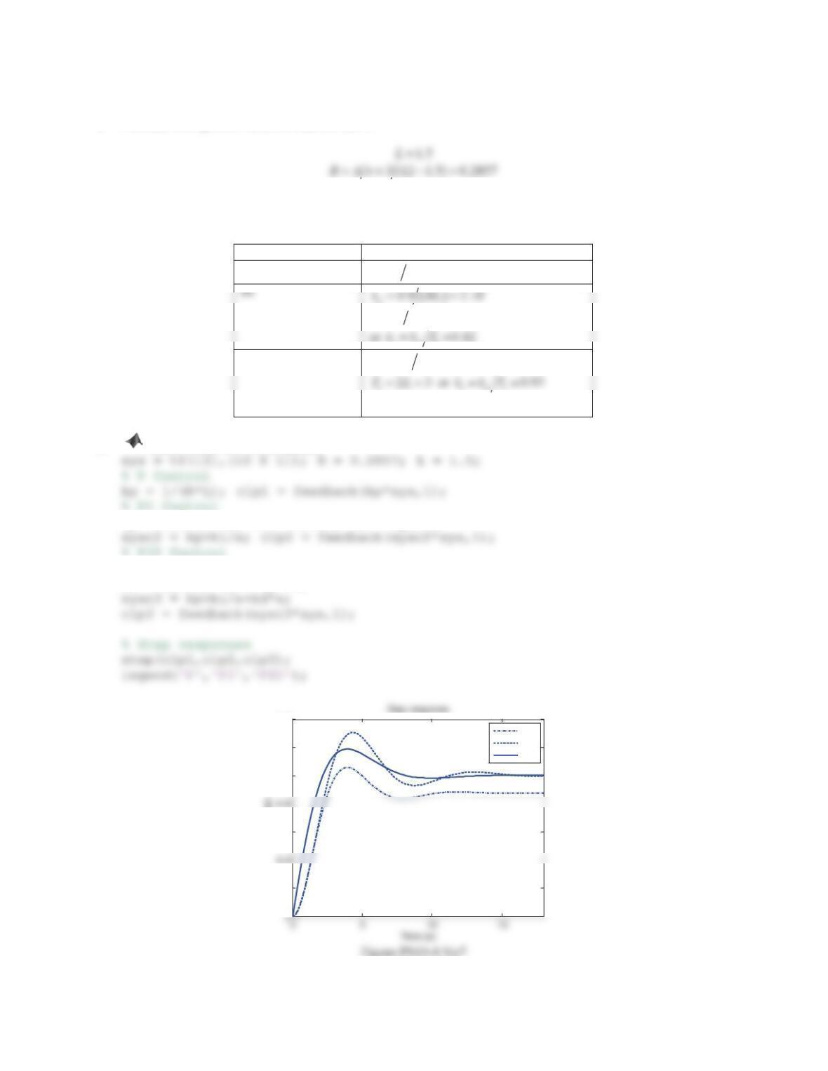
b. Assume that the transfer function of the plant is 3/(10s2+8s+1). Use MATLAB to plot the unit-step
response of the closed-loop system with P, PI, or PID control.
441
Solution
a. Estimate the lag time Land the reaction rate R:
The proportional, PI, and PID controller parameters are listed in the table.
Table PS10-4 No7
Type of controller Optimum gains
P
p
1 2.33kRL
I
0.3 5TL
IpI
PID
p
1.2 2.8kRL
D0.5 0.75TL or
DpD
2.10kkT
b. Below is the MATLAB session.
kp = 0.9/(R*L); Ti = L/0.3; ki = kp/Ti;
kp = 1.2/(R*L); Ti = 2*L; Td = 0.5*L;
ki = kp/Ti; kd = kp*Td;
0.2
0.6
1
1.2
1.4
Amplitude
P
PI
PID
8. Consider a proportional feedback control system. As shown in Figure 10.45, the closed-loop system becomes
marginally stable when the proportional gain is 0.75. Find the P, PI, and PID controller parameters using the
Ziegler–Nichols ultimate sensitivity method.
Figure 10.45 Problem 8.
Solution
The proportional, PI, and PID controller parameters are listed in the table, where
18
u
P|
and
u
K
is given as 0.75.
Table PS10-4 No8
Type of controller Optimum gains
P
pu
0.5 0.375kK
pu
Iu
1.2 15TP
or
IpI
0.0225kkT
Iu
IpI
Du
8 2.25TP
or
DpD
1.0125kkT
Problem Set 10.5
1. Roughly sketch the root locus with respect to Kfor the equation of 1 + KL(s) = 0 and the following choices for
L(s). Make sure to give the asymptotes, arrival and/or departure angles, and points crossing the imaginary axis.
Verify your results using MATLAB.
a.
1
() (1)(3)
Ls ss
b. 1
() (1)(3)(11)
Ls sss
c.
5
() (1)(3)(11)
s
Ls sss
d.
(5)
() (1)(3)(11)
ss
Ls sss
Solution
a. poles:
1
,
3
zeros: none
Asymptotes for large gain values:
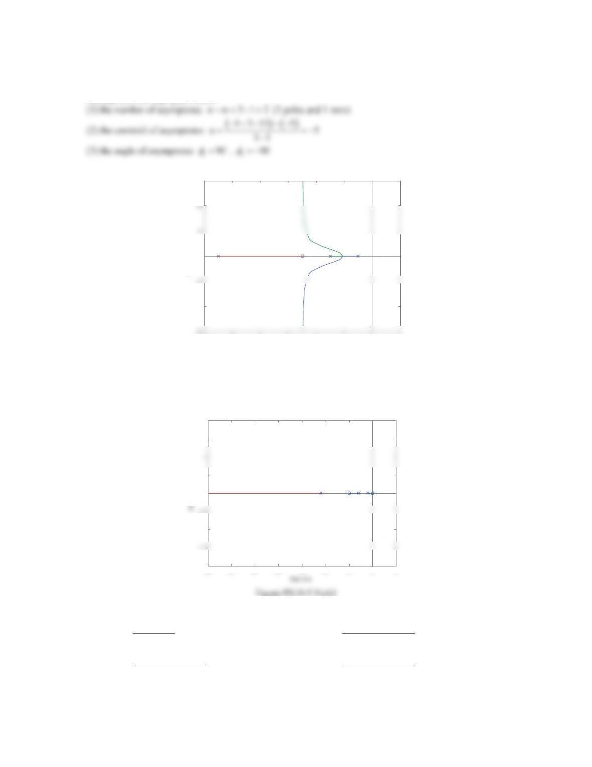
(1) the number of asymptotes: 200nm (2 poles and no zeros)

443
-3.5 -3 -2.5 -2 -1.5 -1 -0.5 00.5
-1.5
-0.5
0.5
2
Root Locus
Real Axis
Figure PS10-5 No1a
b. poles:
1
,
3
,
11
zeros: none
Asymptotes for large gain values:
(1) the number of asymptotes:
30 0nm
(3 poles and no zeros)
(3) the angle of asymptotes: 160
I
D,2180
I
D,
3
60
I
D
Crossing jZ-axis points:
1jȦ
jȦ MȦ MȦ
K
KL
32
Root Locus
Real Axis
Imaginary Axis
-40 -30 -20 -10 010 20
-30
-10
0
10
20
30
Figure PS10-5 No1b
444
c. poles:
1
,
3
,
11
zeros:
5
Asymptotes for large gain values:
-12 -10 -8 -6 -4 -2 0 2
-20
0
30
Root Locus
Real Axis
Imaginary Axis
Figure PS10-5 No1c
d. poles:
1
,
3
,
11
zeros: 0,
5
(Note that all the branches are on the real axis.)
-35 -30 -25 -20 -15 -10 -5 05
-2
-1
0
0.5
1.5
2
Root Locus
2. Repeat Problem 1 for the following choices for L(s).
a. 2
1
() 25
Ls ss b.
2
1
() (4)( 25)
Ls sss
c.
2
2
45
() (4)( 25)
ss
Ls sss
d.
2
2
(1)( 45)
() (4)( 25)
sss
Ls sss

445
Solution
a. poles:
12jr
zeros: none
Asymptotes for large gain values:
(1) the number of asymptotes: 200nm (2 poles and no zeros)
-2 -1.5 -1 -0.5 00.5
-8
-4
0
2
4
6
8
10
Root Locus
Real Axis
Figure PS10-5 No2a
b. poles:
4
,
12jr
zeros: none
Asymptotes for large gain values:
(1) the number of asymptotes:
30 0nm
(3 poles and no zeros)
(3) the angle of asymptotes:
1
60
I
D
,
2
180
I
D
,
3
60
I
D
Departure angle from the complex pole at
1sj
:
which is equivalent to
2
3
6Ȧ
ȦȦ
K
®
¯

446
-8 -7 -6 -5 -4 -3 -2 -1 0 1 2
-6
-2
6
Root Locus
Real Axis
Imaginary Axis
Figure PS10-5 No2b
c. poles:
4
,
12jr
zeros:
2jr
Asymptotes for large gain values:
Departure angle from the complex pole at
12js
:
Arrival angle to the complex zero at
2js
:
-8 -7 -6 -5 -4 -3 -2 -1 0 1
-2.5
-1.5
-0.5
1
1.5
Real Axis
Imaginary Axis
Figure PS10-5 No2c
d. poles:
4
,
12j
r
zeros: 1,
2jr
447
Departure angle from the complex pole at
12js
:
Arrival angle to the complex zero at
2js
:
11
31
arr 12
180 135 180 tan tan 135 90 180 45
ii
MM\
ªºªº
66
¬¼¬¼
DDD DDDD
-4.5 -4 -3.5 -3 -2.5 -2 -1.5 -1 -0.5 00.5
-2.5
-1.5
-0.5
1
1.5
Real Axis
Imaginary Axis
Figure PS10-5 No2d
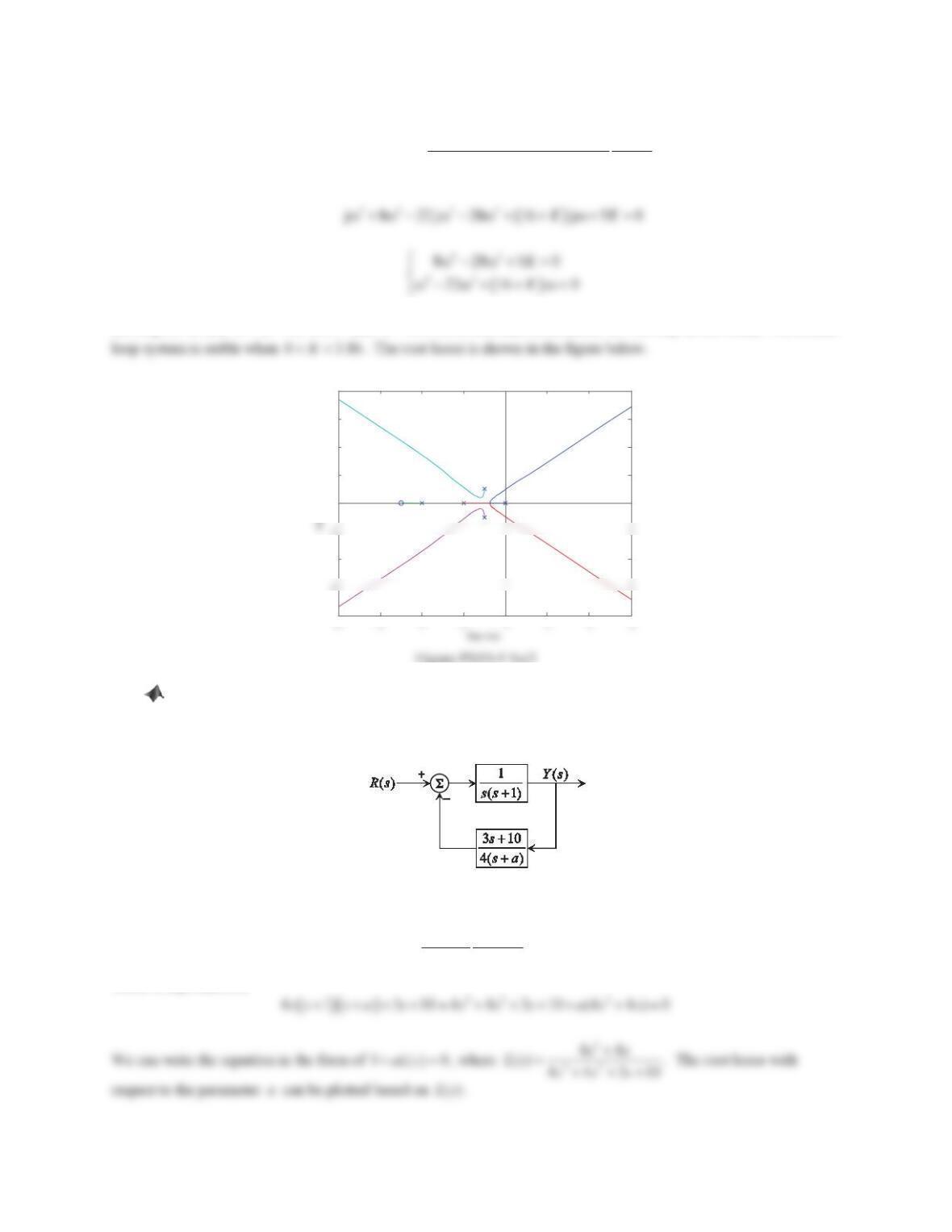
3. A control system is represented using the block diagram shown in Figure 10.57. Sketch the root locus with
respect to the proportional control gain K. Determine all the values of Kfor which the closed-loop system is
stable.
Figure 10.57 Problem 3.
Solution
The closed-loop characteristic equation is
2
51
1()1 0
2
422
s
KL s K s
ss s s
Poles of
()Ls
: 0,
2
,
4
,
1jr
zero of
()Ls
:
5
Asymptotes for large gain values:
(3) the angle of asymptotes:
1
45
I
D
,
2
135
I
D
,
3
135
I
D
,
4
45
I
D
Departure angle from the complex pole at
1js
:
448
Crossing jZ-axis points:
2
jȦ
1jȦ
jȦ
jȦMȦ MȦ MȦ
KL K
ªº
¬¼
Solving for Ȧand
K
:
Ȧ
,0.97rand 0K , 3.86 (Note that the solution,
5.32 j
Z
r
is not valid). The closed-
-8
-4
0
2
4
6
8
Root Locus
4. A control system is represented using the block diagram shown in Figure 10.58, where the parameter ais
subjected to variations. Use MATLAB to plot the root locus with respect to the parameter a. Determine all the
values of afor which the closed-loop system is stable.
Figure 10.58 Problem 4.
Solution
The closed-loop characteristic equation is
1310
10
14( )
s
ss s a
which is equivalent to
449
Below is the MATLAB session.
>> L = tf([4 4 0],[4 4 3 10]); rlocus(L);
-3.5 -3 -2.5 -2 -1.5 -1 -0.5 00.5
-1.5
-0.5
0.5
Real Axis
Figure PS10-5 No4
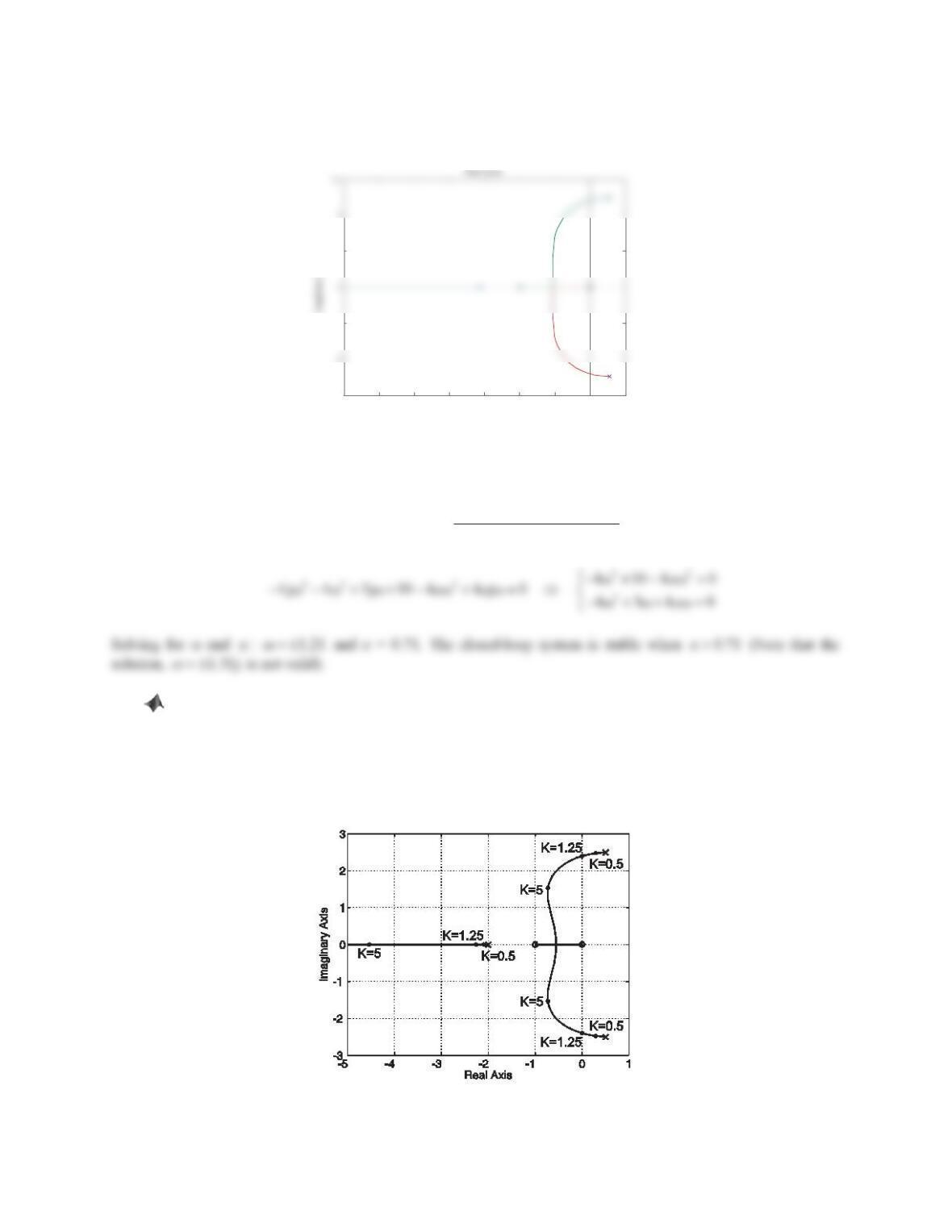
The stability range of acan be determined by fining the crossing jZ-axis points.
2
32
4( jȦ MȦ
1jȦ
4( jȦ MȦ MȦ
aL a
5. Figure 10.59 shows the root locus of a unity negative feedback control system, where Kis the proportional
control gain.
a. Determine the transfer function of the plant. Use MATLAB to plot the root locus based on your choice of
the plant, compare it with the root locus shown in Figure 10.59, and check the accuracy of your plant.
b. Give comments on the stability of the closed-loop system when Kvaries from 0 to .
c. Give comments on the transient performance of the closed-loop system when K= 0.5 and 5. Use MATLAB
to plot the corresponding unit-step responses and verify your comments.
Figure 10.59 Problem 5.
450
Solution
a. Note that there are three branches. Two of them end at zeros and the other ends at infinity. This implies that the
plant is a third–order system and has two zeros. When 0K , which corresponds to having no control, three
poles are located at
2
,
0.5 2.5jr
and two zeros are at 0, 1. Thus, a possible transfer function of the plant is
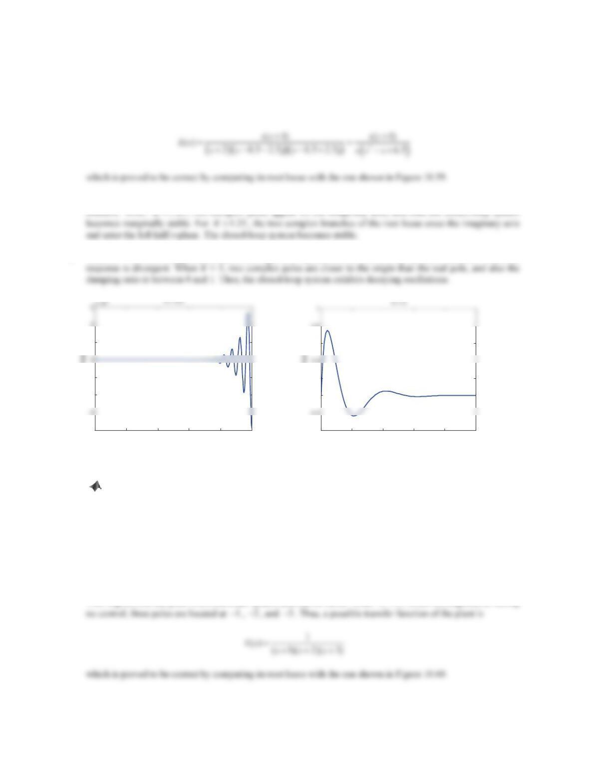
b. When 0 1.25Kd , two complex poles are in the right half s-plane, and thus the closed-loop system is
c. When K= 0.5, two complex poles are in the right half s-plane and the closed-loop system is unstable. Thus, the
010 20 30 40 50
-4
-2
-1
1
Time (s)
Closed–loop response
0 2 4 6 8 10
-0.4
0
0.2
0.6
0.8
Time (s)
Closed-loop response
Figure PS10-5 No5
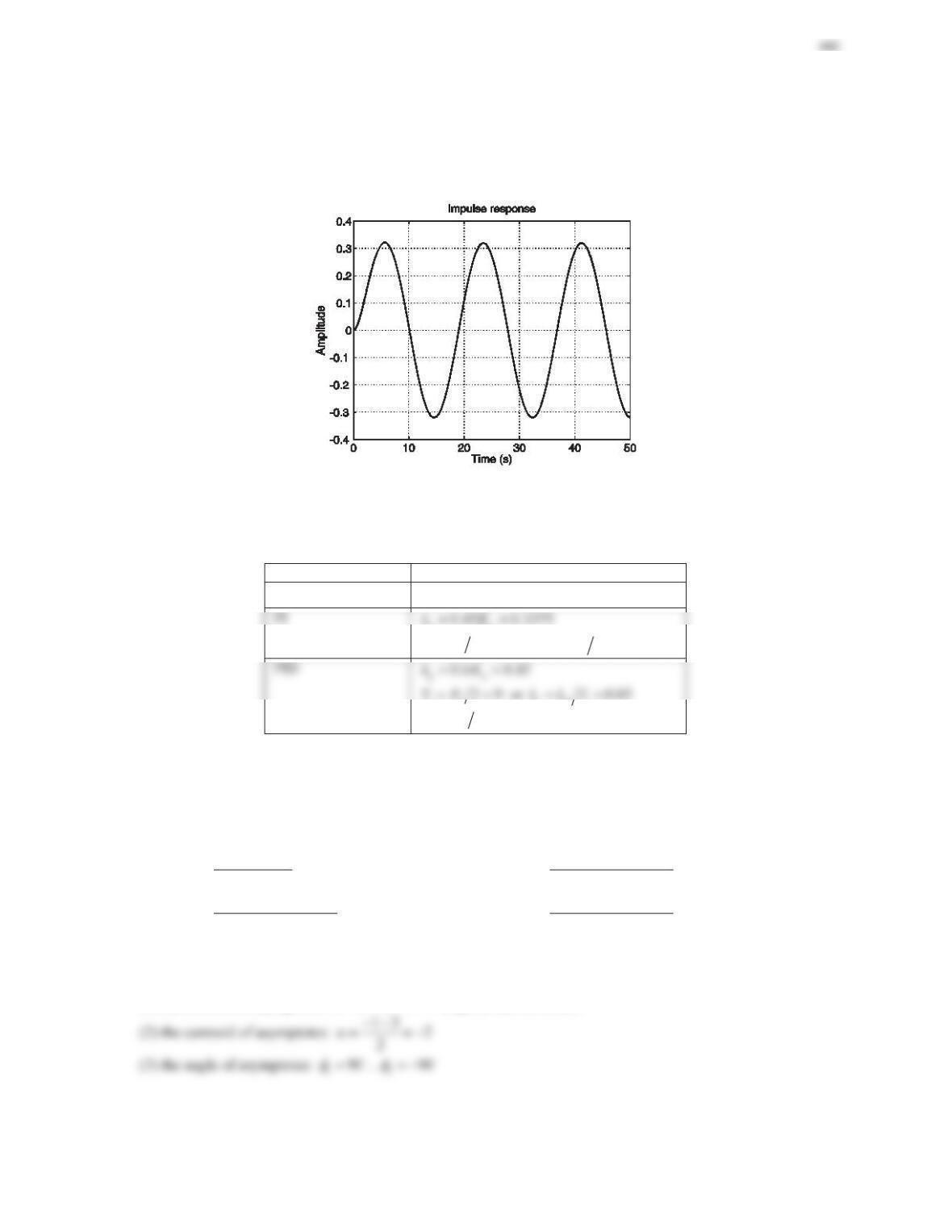
6. Figure 10.60 shows the root locus of a unity negative feedback control system, where Kis the proportional
control gain.
a. Determine the transfer function of the plant. Use MATLAB to plot the root locus based on your choice of
the plant, compare it with the root locus shown in Figure 10.60, and check the accuracy of your plant.
b. Find the range of values of Kfor which the system has damped oscillatory response. What is the greatest
value of Kthat can be used before pure harmonic oscillations occur? Also, what is the frequency of pure
harmonic oscillations? Use MATLAB to plot the corresponding unit-step response and verify the accuracy
of your computed frequency.
Solution
a. Note that there are three branches, all of which start at poles and end at infinity by approaching to asymptotes.
This implies that the plant is a third-order system and has no zeros. When 0K , which corresponds to having
451
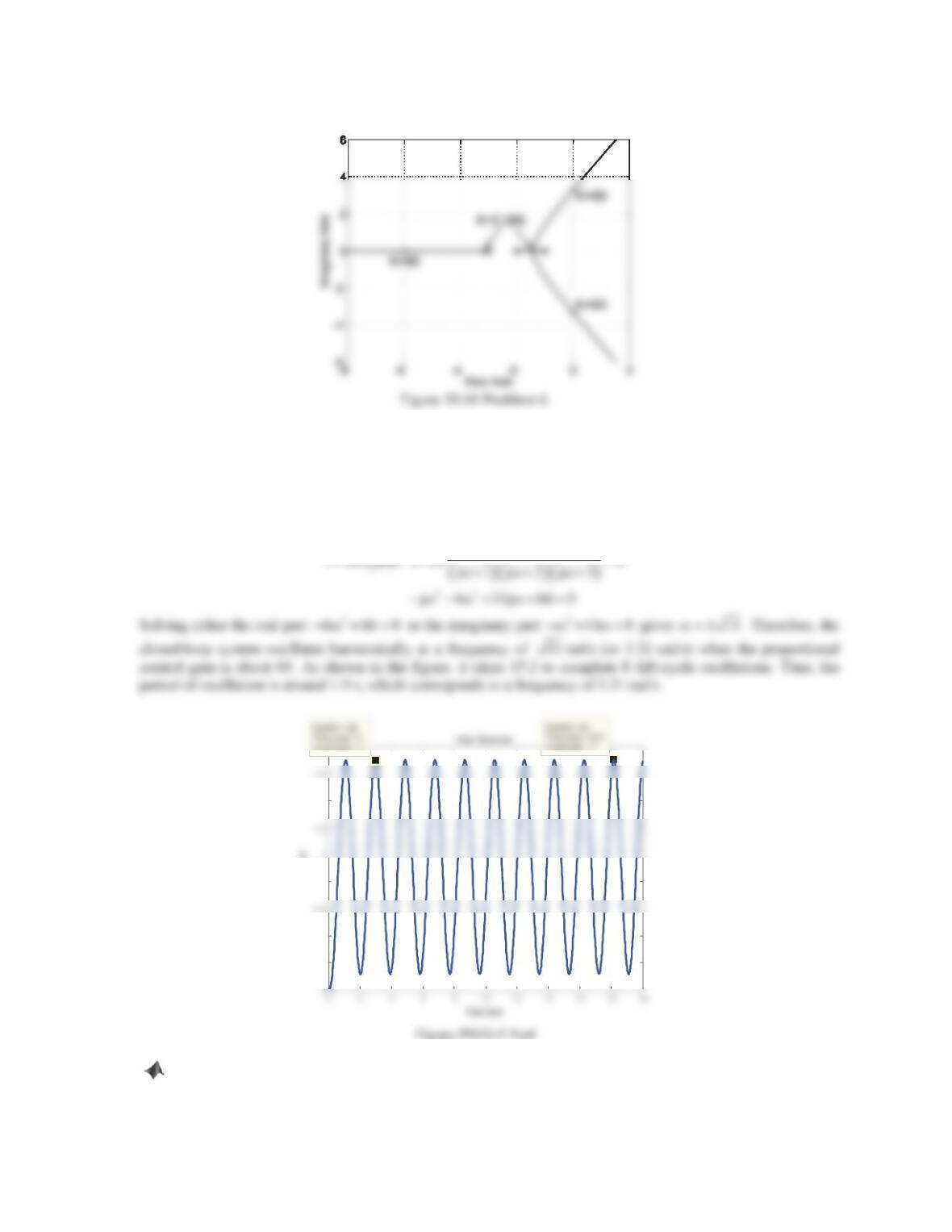
b. Note that the root loci starting at
1
and
2
break away from the real axis when
0.385K
and the poles split
into a complex conjugate pair when 0.385K!. These two complex branches cross the imaginary axis into the
right half s-plane when
60K
. Thus, the closed-loop system has damped oscillatory response when
0.385 60K. The greatest value of
K
which can be used before pure harmonic oscillations occur is about
60. The frequency of pure harmonic oscillations can be determined by solving for the crossing jZ-axis points.
We have
1
Amplitude
0.2
0.4
0.8
1.4
7. Consider the feedback system shown in Figure 10.61.
a. Find the locus of the closed-loop poles with respect to K.
452
b. Find a value of Ksuch that the maximum overshoot in the response to a unit-step reference input is less
than 10%. What is the corresponding steady-state error of the closed-loop system?
c. Plot the unit-step response of the closed-loop system to verify the result for Part (b).
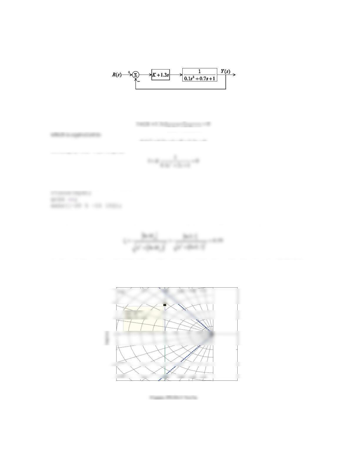
Figure 10.61 Problem 7.
Solution
a. The characteristic equation of the closed-loop system is
0.1 0.7 1
ss
0.1 0.7 1 1.3 0ssKs
Dividing by
2
0.1 2 1ss
gives
which is in the form of
1()0KL s
. We can plot the root locus based on
()Ls
.
sys = tf([1],[0.1 2 1]);
b. The requirement for the transient response of the closed-loop system is
p
10%M
. This implies that
As shown in the root locus, the dashed diagonal lines indicate pole locations with a damping ratio of 0.59. Only
the part of the root locus in between the two diagonal lines is acceptable. Choose
18K
.
Root Locus
Real Axis
-20 -15 -10 -5 0 5
-15
-5
0.91
0.975
0.975
Damping: 0.725
Overshoot (%): 3.67
453
c. The following is the MATLAB session.
K = 18; sysc = tf([1.3 K],[1]); sys = tf([1],[0.1 0.7 1]);
S t ep Res ponse
Time (sec)
00.1 0.2 0.3 0.4 0.5 0.6 0.7 0.8 0.9 1
0.4
1
1.2
1.4
Overshoot (%): 9.39
At time (sec): 0.21
Figure PS10-5 No7b
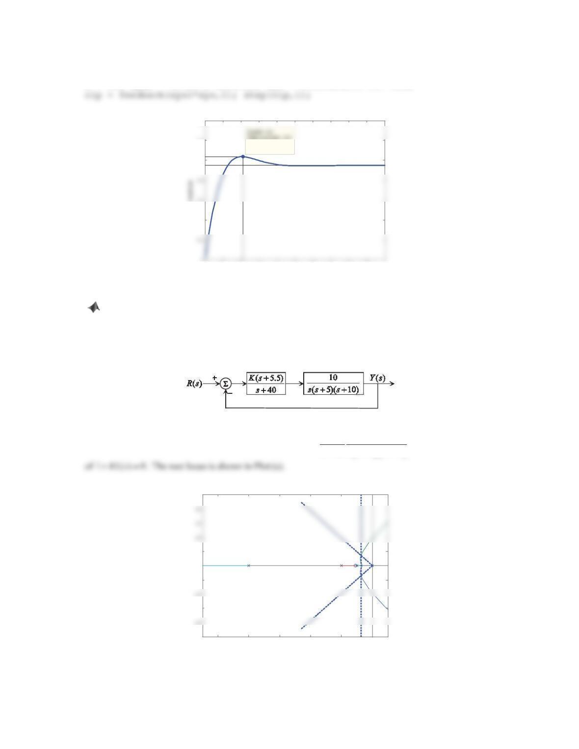
8. Consider the feedback system shown in Figure 10.62.
a. Find the locus of the closed-loop poles with respect to K.
b. Find a value of Ksuch that the maximum overshoot in the response to a unit-step reference input is less
than 20% and the 2% settling time is less than 1.1 s.
c. Plot the unit-step response of the closed-loop system to verify the result in Part (b).
Figure 10.62 Problem 8.
Solution
a. The characteristic equation of the closed-loop system is
5.5 10
10
40 5 10
s
Kssss
, which is in the form
-50 -40 -30 -20 -10 0
-50
-30
-10
0
10
50
Root Locus
Real Axis
Imaginary Axis
Figure PS10-5 No8a
454
Root Locus
Real Axis
-6 -5 -4 -3 -2 -1 0 1
-8
-4
0
6
8
10
Damping: 0.674
Overshoot (%): 5.69
Figure PS10-5 No8b
b. The requirements for the transient response of the closed-loop system are overshoot
p
20%M
and 2% settling
time
1.1
s
t
s. This implies that
p
22
2
2
p
ln ln 0.20
ȗ
ʌ OQ
ʌOQ
M
M
!
c. The following is the MATLAB session. The closed-loop step response is shown in Plot (c).
K = 150; sysc = tf(K*[1 5.5],[1 40]); sys = tf([10],conv([1 5 0],[1 10]));
clp = feedback(sysc*sys,1); step(clp,2);
Step Response
Time (sec)
Amplitude
00.2 0.4 0.6 0.8 11.2 1.4 1.6 1.8 2
0
0.2
0.6
0.8
1.4
System: clp
Peak amplitude: 1.07
455
Problem Set 10.6
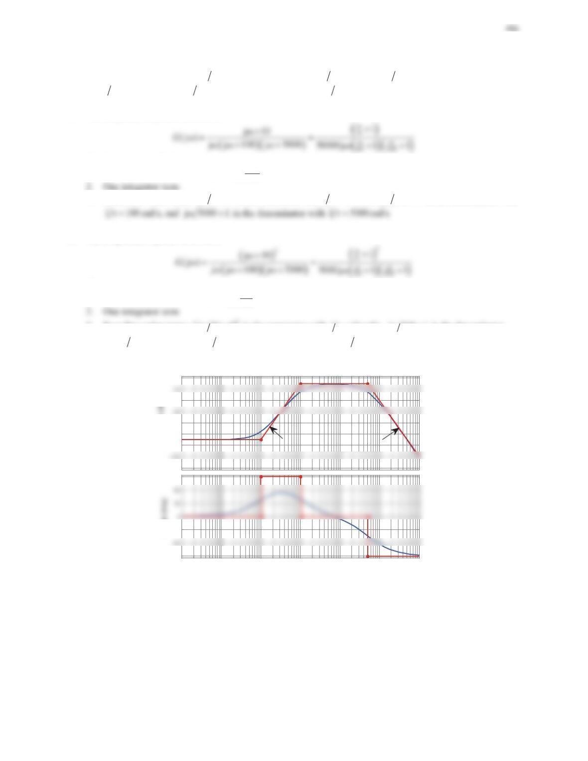
1. Sketch the asymptotes of the Bode plot magnitude and phase for the following open-loop transfer functions.
Make sure to give the corner frequencies, slopes of the magnitude plot, and phase angles. Verify the results
using MATLAB.
a.
10
() 100
s
Gs s
b.
10
() ( 100)( 5000)
s
Gs ss
c.
10
() ( 100)( 5000)
s
Gs ss s
d.
2
(10)
() ( 100)( 5000)
s
Gs ss s
Solution
a. The frequency response function is
The basic terms include:
2. Two first–order terms:
jȦ
in the numerator with 1IJ rad/s and jȦ in the denominator
with
1IJ
rad/s
Bode Diagram
Frequency (rad/sec)
-20
-12
-4
0
0.1 1 10 100 1000 10000
75
90
Figure PS10-6 No1a
b. The frequency response function is
100 5000
The basic terms include:
2. Three first-order terms: jȦ in the numerator with
1IJ
rad/s, jȦ in the denominator with
1IJ
rad/s, and jȦ in the denominator with 1IJ rad/s
c. The frequency response function is
The basic terms include:
1. One constant term 1/50000 ( 1
10 50000
20log 94 dB)
3. Three first-order terms:
jȦ
in the numerator with
1IJ
rad/s, jȦ in the denominator with
d. The frequency response function is
The basic terms include:
1. One constant term 1/5000 (
1
10 5000
20log 74
dB)
3. Four first-order terms:
jȦ in the numerator with
1IJ
rad/s, jȦ in the denominator
with
1IJ
rad/s, and jȦ in the denominator with 1IJ rad/s
Bode Diagram
Frequency (rad/sec)
-104
-96
-92
-88
-80
-72
Magnitude (dB)
0.1 1 10 100 1000 10000 100000
-90
-30
90
Phase (deg)
20 dB/dec –20 dB/dec
Figure PS10-6 No1b
457
Frequency (rad/sec)
-220
-200
-160
-120
-80
0.1 1 10 100 1000 10000 100000
-180
-120
-60
0
Phase (deg)
-40 dB/dec
-20 dB/dec
Figure PS10-6 No1c
Bode Diagram
-104
-96
-84
-76
-72
-45
90
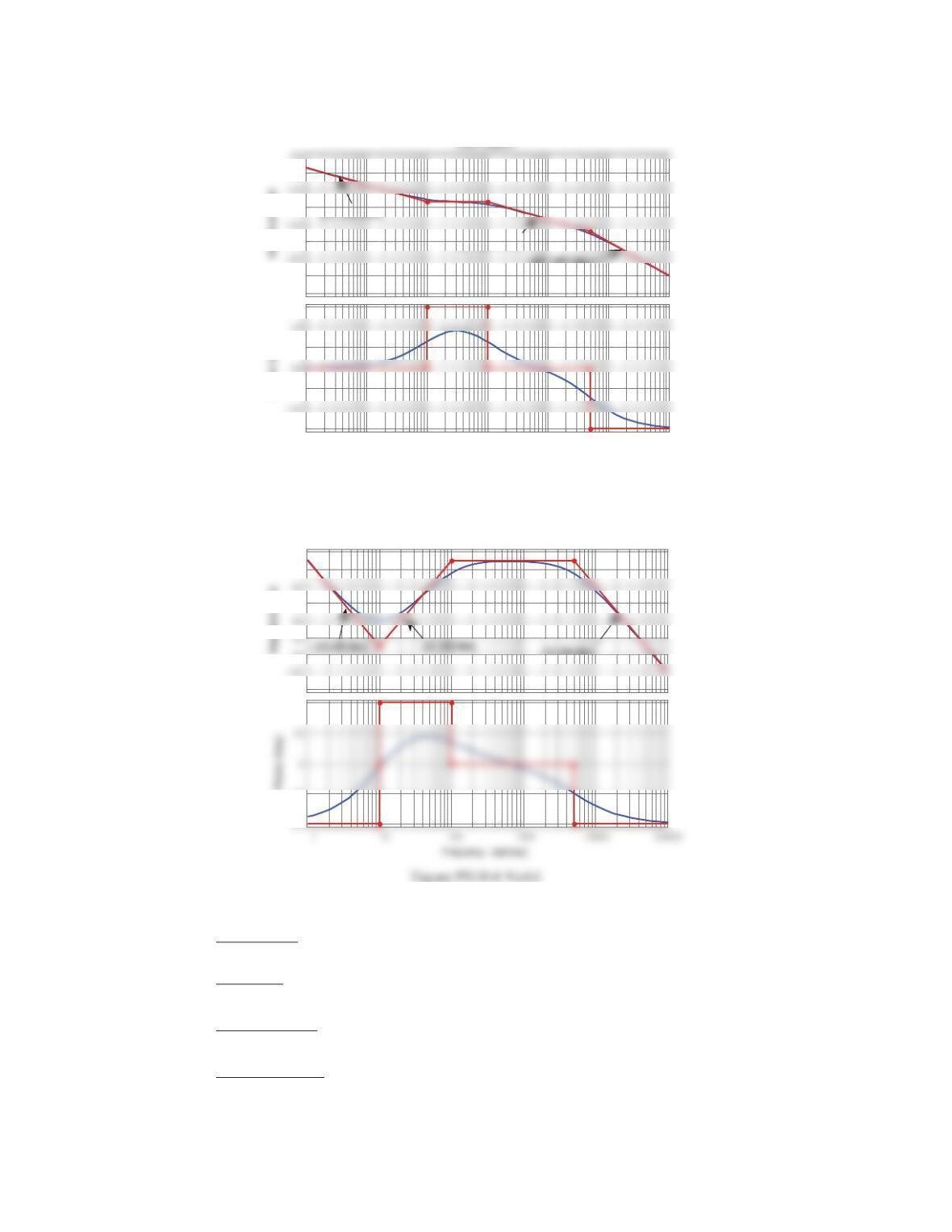
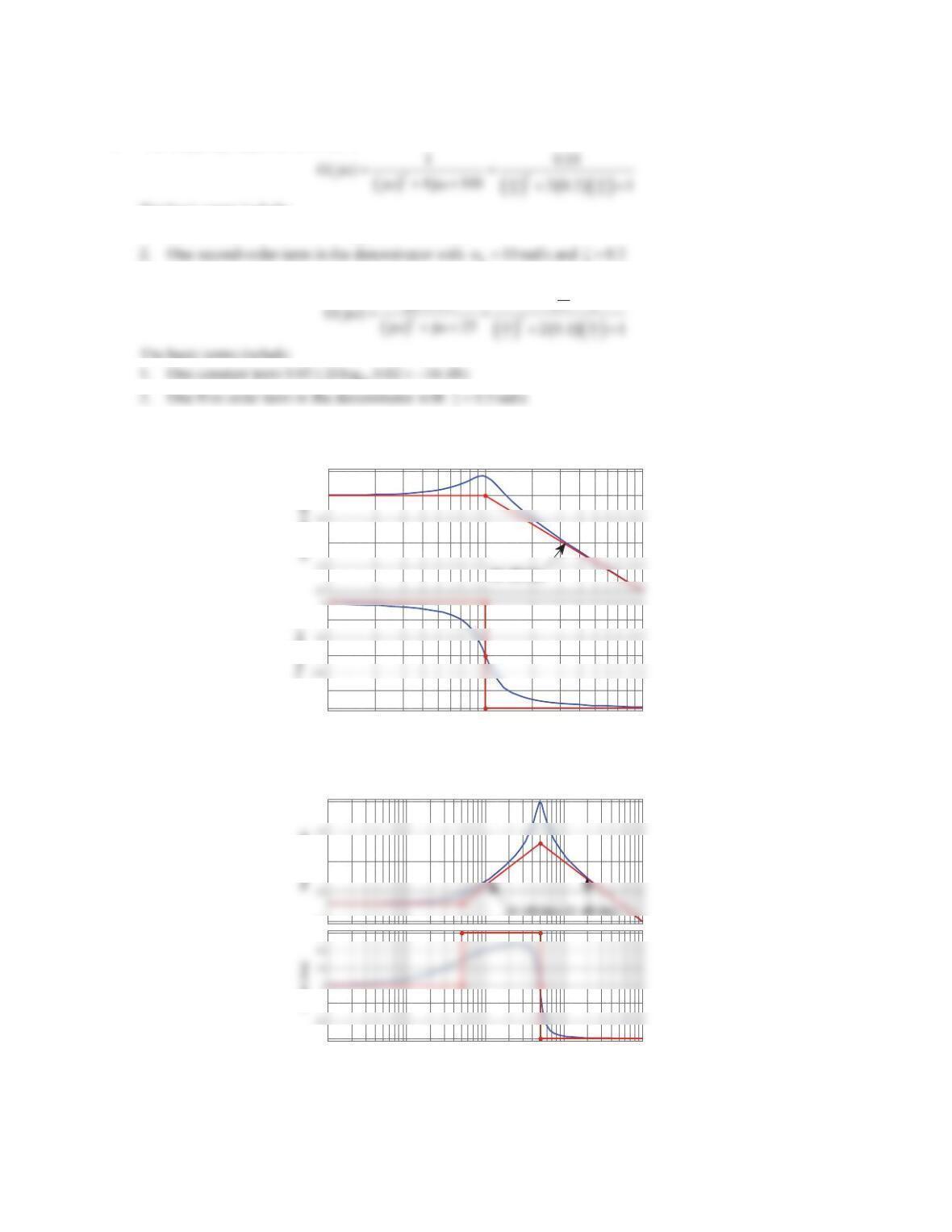
2. Repeat Problem 1 for the following open-loop transfer functions.
a.
2
1
() 4 100
Gs ss
b.
2
0.
() 25
5
Gs ss
s
c.
2
2
0.1 25
() 0.24 144
ss
Gs ss
d.
2
100( 7 49)
() ( 1)( 500)
ss
Gs ss
458
Solution
a. The frequency response function is
The basic terms include:
1. One constant term 0.01 ( 10
20log 0.01 40 dB)
n
b. The frequency response function is
jȦ
0.5
0.02 1
jȦ
3. One second-order term in the denominator with
n
Ȧ
rad/s and
ȗ
Bode Diagram
Frequency (rad/sec)
-60
-40
-30
1 10 100
-180
-150
-90
-30
-40 dB/dec
Figure PS10-6 No2a
Bode Diagram
Frequency (rad/sec)
-40
-20
0
0.01 0.1 1 10 100
-90
-30
90
Phase (deg)
Figure PS10-6 No2b