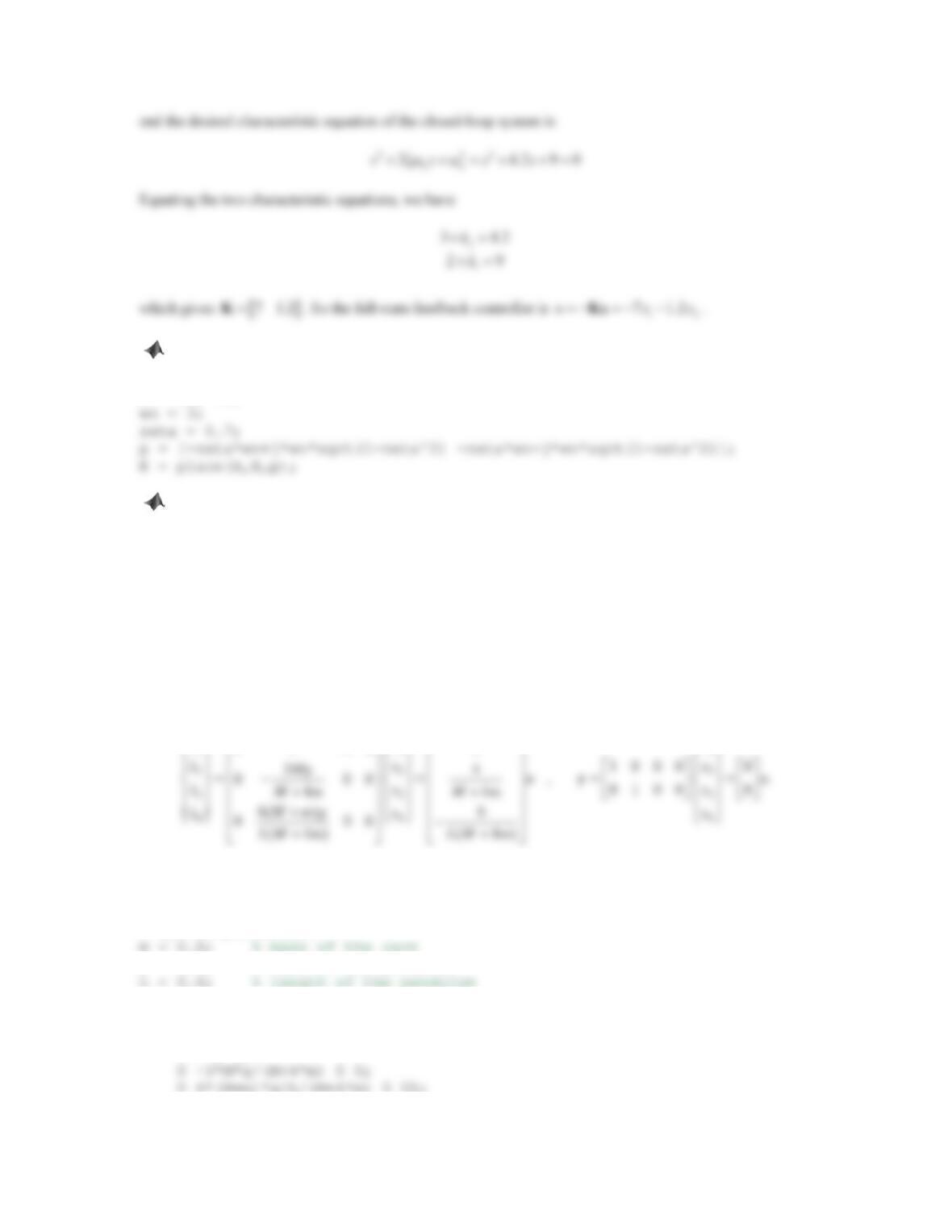
8. Consider Problem 7 in Problem Set 10.7. Using the full-state feedback controller obtained in Part (b), build
a Simulink block diagram to simulate the resulting feedback control system. Find the closed-loop response if
the initial conditions are x1(0) = 0.1 and x2(0) = 0.
00.5 11.5 2
0
0.02
0.06
0.1
Time (s)
Figure PS10-8 No8b
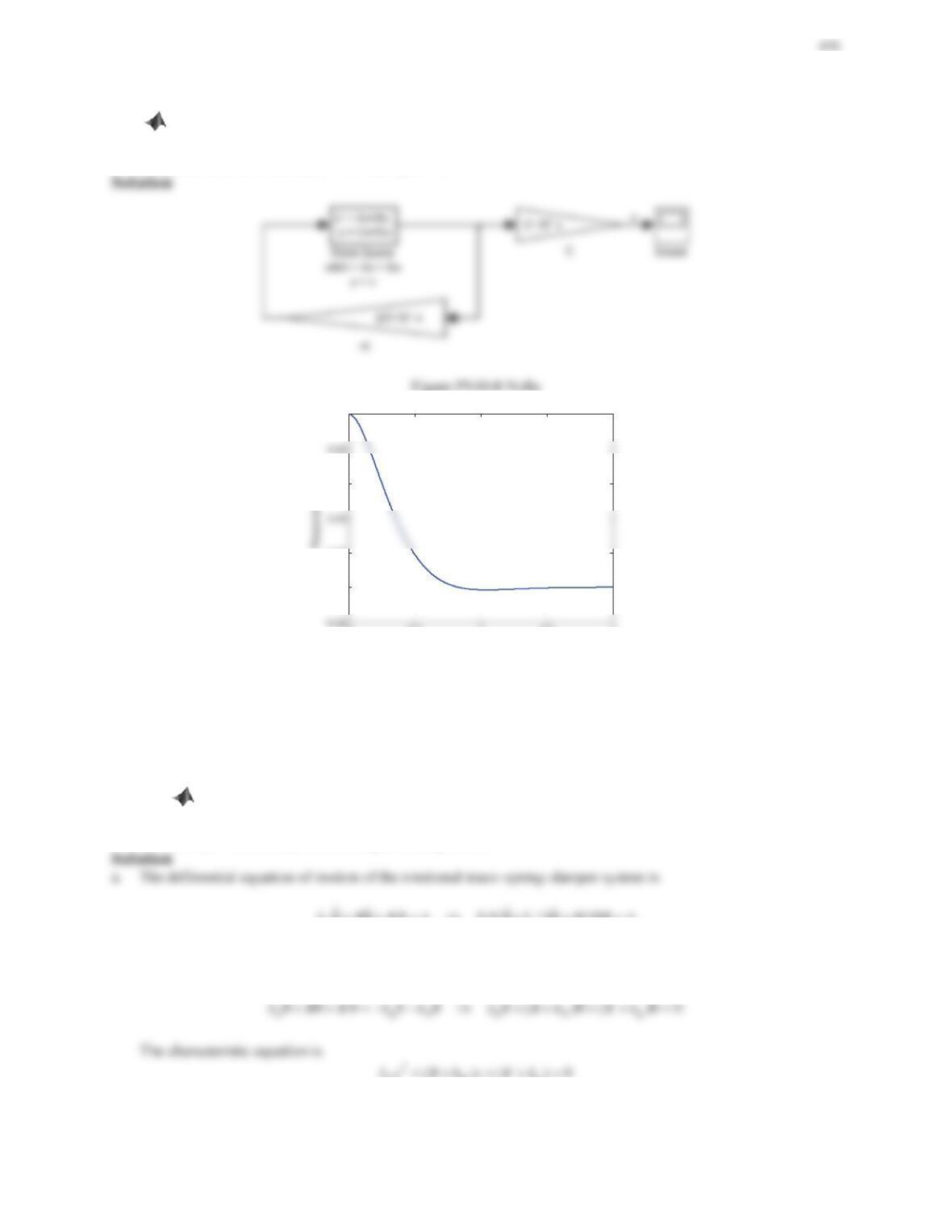
9. Consider the rotational mass–spring–damper system in Example 5.20. A PD controller, pD
IJșșkk , is
designed to adjust the input torque Wso that the rotational disk can quickly return to the equilibrium position
regardless of disturbances applied to the system. The performance requirements of the closed-loop system are
overshoot Mp< 5% and rise time tr< 0.004 s.
a. Design a PD controller to meet the performance requirements.
b. Build a block diagram of the feedback control system, where the plant is constructed using Simscape
blocks and the controller is constructed using Simulink blocks. Find the closed-loop response if the disk is
initially 0.1 rad away from the equilibrium position.
O
0.01 1.15 4150IBKT T T W T T T W
For a feedback control system with a PD controller pD
IJșșkk , the differential equation of motion of the
closed-loop system is
ODp
1.12 0.078 2.230 1.12 0.078(0.69) 2.230(0.69) 532
]]
n
n
ȗ
p750k
and
D
10.05k
.
b. The block diagram is given in Plot (a), and Plot (b) shows the resulting closed-loop response.
10.05
Converter
RC
Mechanical
Mechanical
du/dt
00.005 0.01 0.015 0.02
0
0.02
0.06
0.1
T(t)
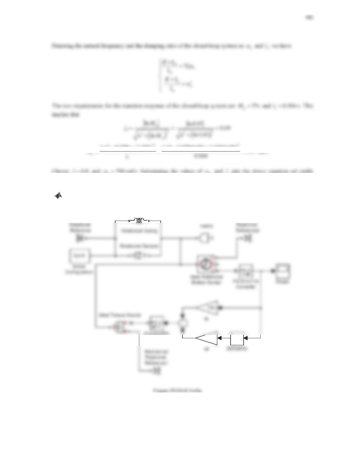
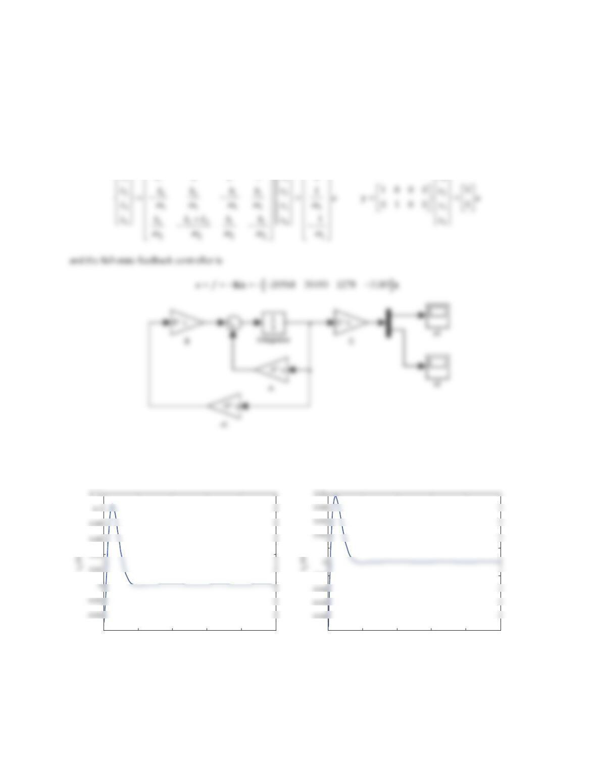
10. Consider the mass–spring–damper system shown in Figure 5.118 (Problem Set 5.6, Problem 3). Assume
that fis a control force to maintain the system at equilibrium regardless of disturbances applied to the system.
a. Design a full-state feedback controller such that the closed-loop poles are located at 10±10j, 15, and 16.
Assume the state vector
1212
[]
T
xx xx x
.
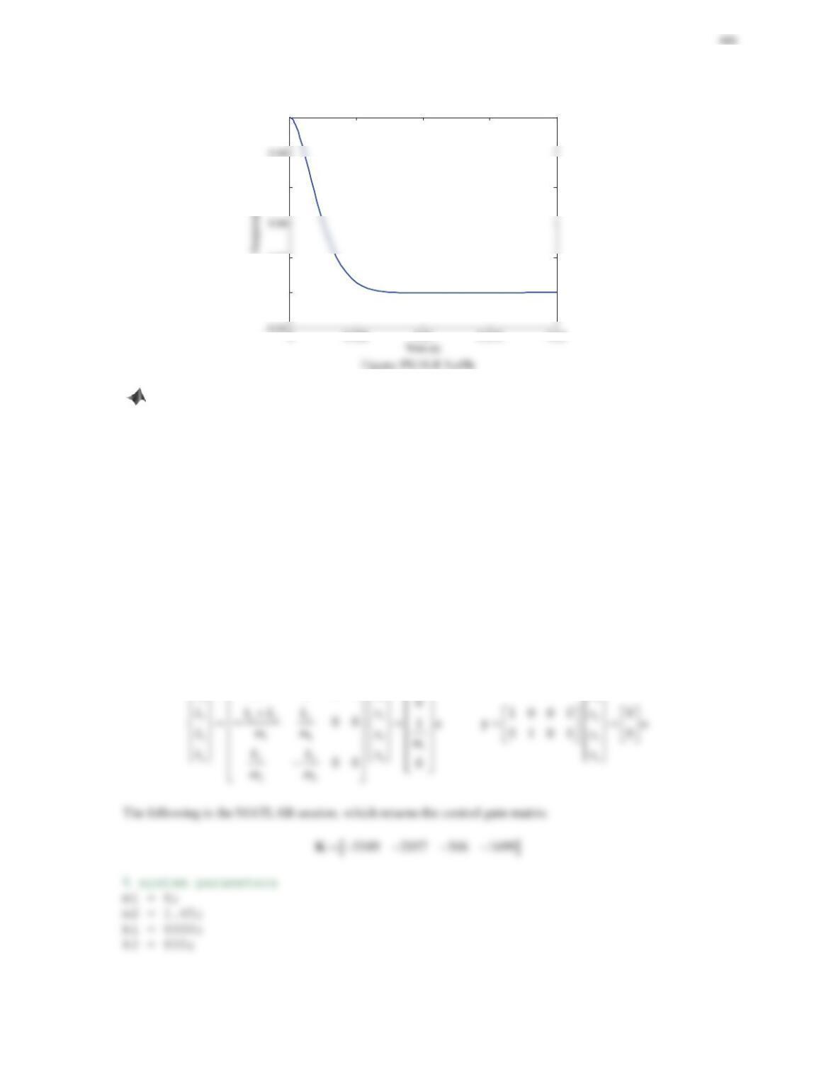
b. Build a Simulink block diagram of the feedback control system. Find the closed-loop response if mass 1 is
initially 0.1 m from the equilibrium position.
Solution
a. The differential equations of motion of the system is
11 1 2 1 2 2
()mx k k x k x f
22 21 22
0mx kx kx
Assume the state vector
1212
[]
T
xx xx x
. Converting to the state-space form yields
11
0010 0
0001 0
xx
ªº
ªº
«»
½ ½«»
x
½
482
% state-space matrices
A = [0 0 1 0;
0 0 0 1;
b. The block diagram is given in Plot (a), and Plot (b) shows the resulting closed-loop response.
x1
x’ = Ax+Bu
y = Cx+Du
State-Space
C* u
C
-K
Figure PS10-8 No10a
00.5 11.5 2
-0.02
0.12
0.18
Time (s)
00.5 11.5 2
-1.5
0.5
2
Time (s)
Figure PS10-8 No10b
Review Problems
1. Consider the feedback control system as shown in Figure 10.87. Determine the range of Kfor closed-loop
stability.
Figure 10.87 Problem 1.
483
Solution
The closed-loop transfer function () ()Ys Rs is
2
43 2
2
2
615
() 2
2
() 11 29 11 2 30
1615
s
Kss s
Ys Ks K
s
Rs ss sK sK
Kss s
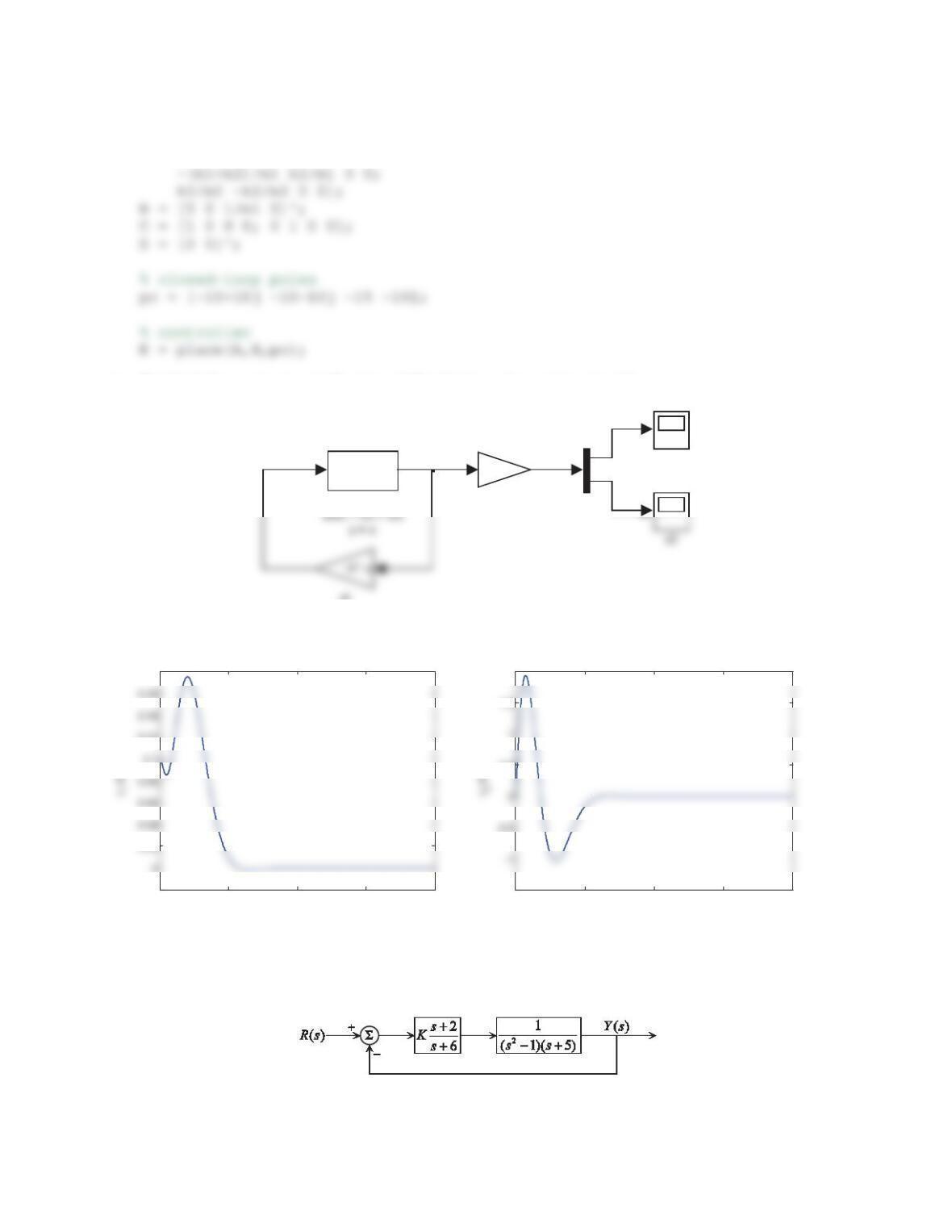
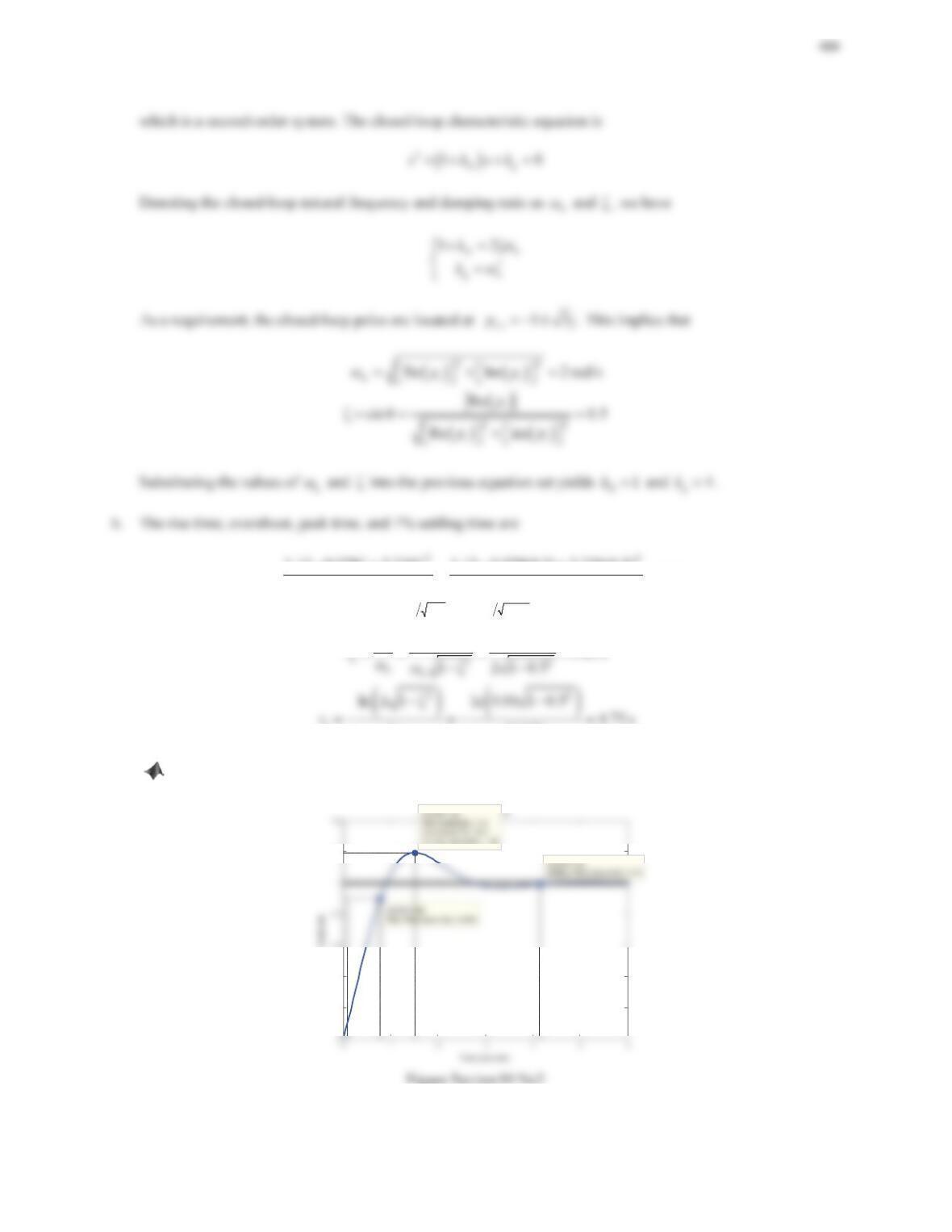
2. Consider the feedback control system shown in Figure 10.88.
a. Design a PD controller such that the closed-loop poles are at 1,2 13jp r .
b. Estimate the rise time, overshoot, peak time, and 1% settling time for the unit-step response of the closed-
loop system.
c. Use MATLAB to plot the unit-step response of the closed-loop system. Verify the answers obtained in
Part (b).
Figure 10.88 Problem 2.
Solution
a. The closed-loop transfer function () ()Ys Rs is
pD
pD
2
Dp
pD
1
1
()
1
() 1
11
kks kks
ss
Ys
Rs sksk
kks
ss
r
n
1.12 0.078 2.230 1.12 0.078(0.5) 2.230(0.5) 0.82
2
t]]
|
Z
s
22
ʌȗ ȗ 0.5ʌ
p
e e 16.30%M
ʌʌ ʌ
s
n
0.5(2)
]Z
c. The unit step response of the closed-loop system is shown in the figure below.
0.2
0.4
1.2
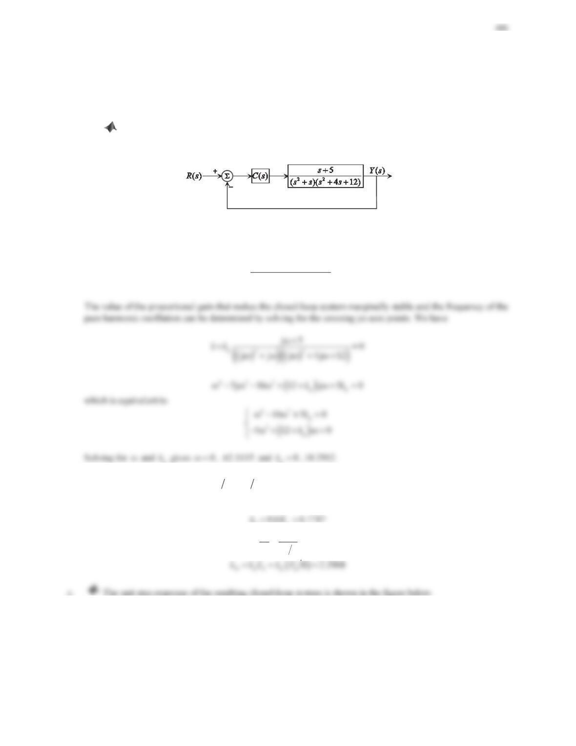
3. Consider the feedback control system as shown in Figure 10.89.
a. Assuming C(s) = kp, determine the value of the proportional gain that makes the closed-loop system
marginally stable. Find the frequency of the sustained oscillation.
b. Using the gain and the frequency obtained in Part (a), apply the ultimate sensitivity method of Ziegler–
Nichols tuning rules to design a PID controller.
c. Plot the unit-step response of the resulting closed-loop system. Find the values of the rise time tr,
overshoot Mp, peak time tp, and 1% settling time ts.
Figure 10.89 Problem 3.
Solution
a. The closed-loop characteristic equation is
p22
5
10
412
s
ksss s
p
p
b. The period of oscillation is
u
2ʌ Ȧ ʌ P
s and the ultimate gain u
Kis 10.2912. Using the
ultimate sensitivity method of Ziegler-Nichols tuning rules, we can determine the PID control gains, which are
pu
pp
I
Iu
4.1501
2
kk
kTP
486
Step Response
Amplitude
0.2
0.4
0.8
1.4
1.8
System: clp
Peak amplitude: 1.63
Overshoot (%): 62.6
At time (sec): 1.85
System: clp
Rise Time (sec): 0.625
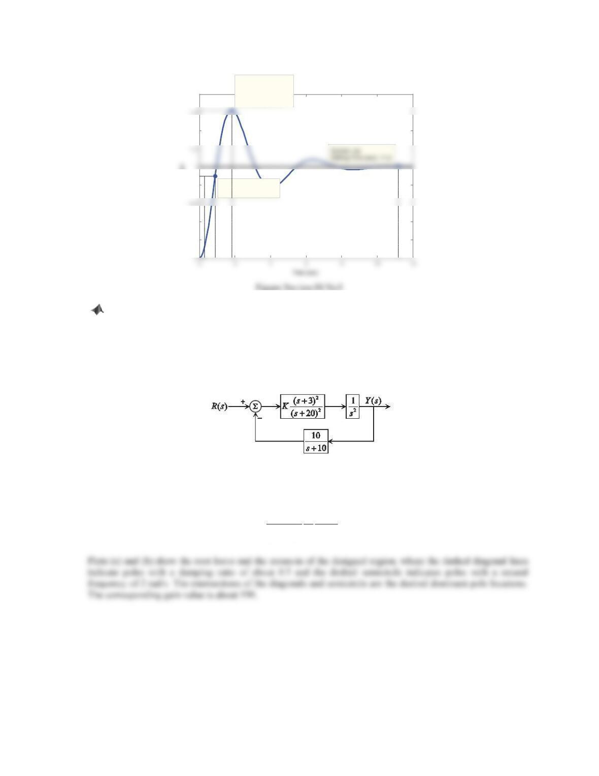
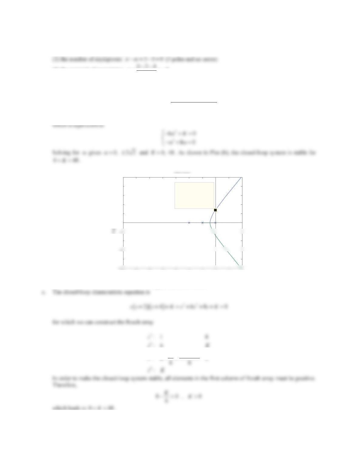
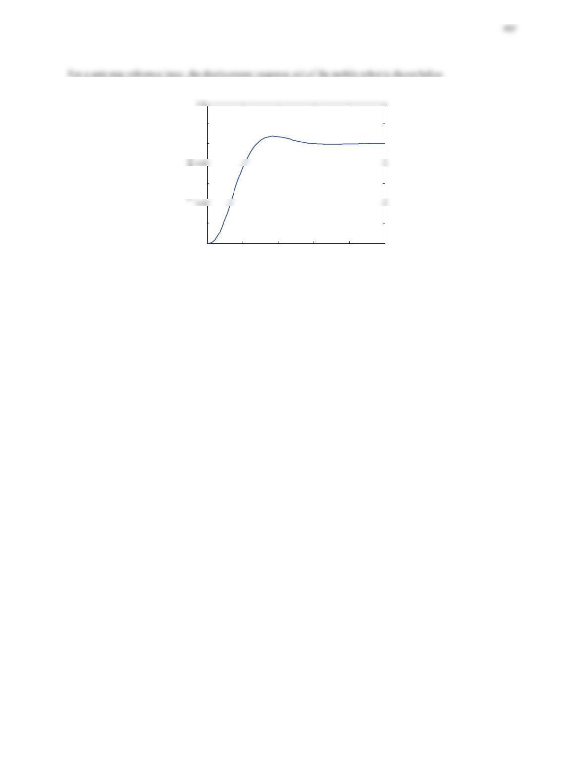
4. Consider the feedback control system as shown in Figure 10.90.
a. Determine the value of the gain KVXFKWKDWWKHXQGDPSHGQDWXUDOIUHTXHQF\ȦnDQGWKHGDPSLQJUDWLRȗRI
the dominant closed-loop poles are around 2 rad/s and 0.5, respectively.
b. Determine the values of all closed-loop poles.
c. Plot the unit-step response of the resulting closed-loop system. Find the values of the rise time tr, overshoot
Mp, peak time tp, and 1% settling time ts.
Figure 10.90 Problem 4.
Solution
a. The closed-loop characteristic equation is
2
22
3110
10
10
20
s
Kss
s
487
-60 -50 -40 -30 -20 -10 010
-20
0
30
Root Locus
Real Axis
Imaginary Axis
Figure Review10 No4a
-5 -4.5 -4 -3.5 -3 -2.5 -2 -1.5 -1 -0.5 0
-3
-1
Real Axis
Figure Review10 No4b
b. The two dominant poles are about
22
1,2 n n
ȗȦ MȦ ȗ M Mp r | r r
Using MATLAB function rlocfind, we can determine the values of the closed-loop poles.
>> p = -1+j*1.732;
>> [K,poles] = rlocfind(sysc*sys*sysh,p)
K =
-28.9837
-9.5045 + 7.6418i
-1.0037 – 1.7241i
c. The unit-step response of the closed-loop system with 190.63K is shown in Plot (c).
Amplitude
00.5 11.5 22.5 33.5 44.5
0
0.2
0.6
0.8
1.2
1.4
At time (sec): 1.06
Rise Time (sec): 0.306
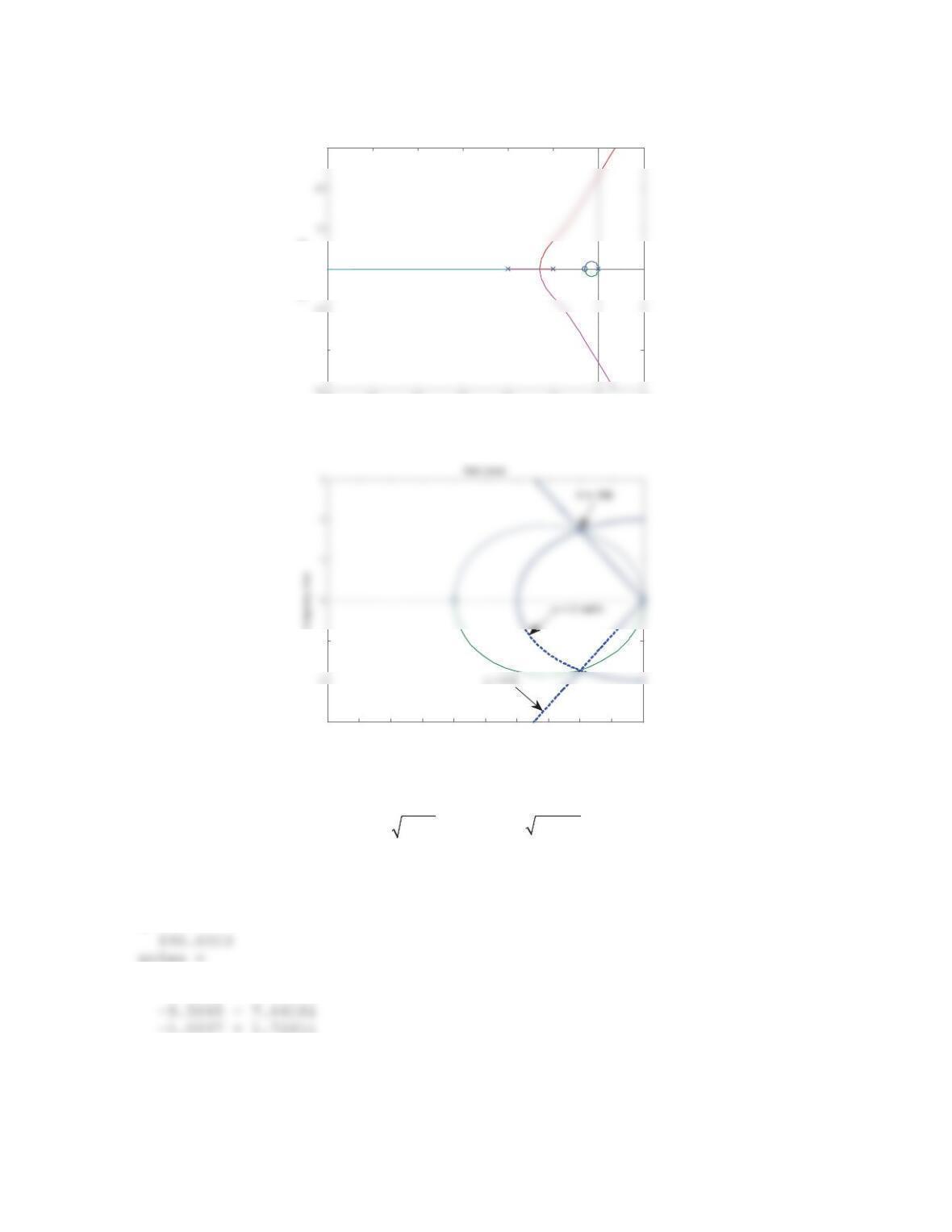
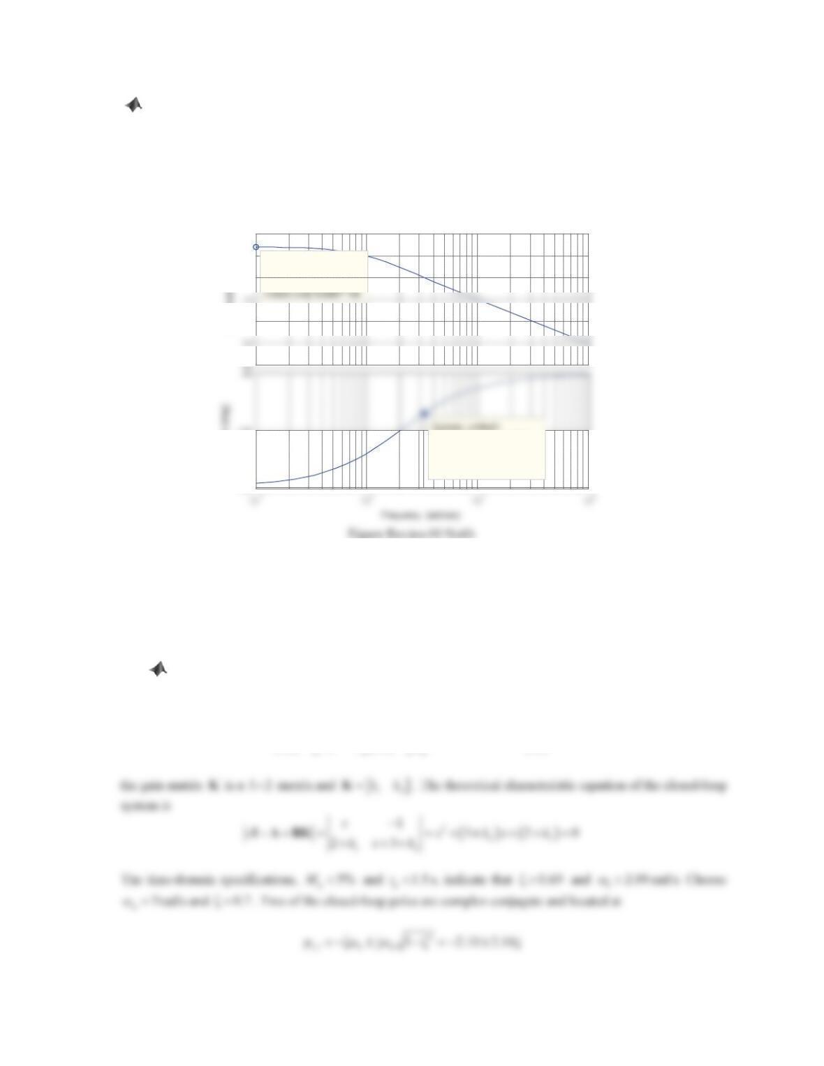
5. Consider a unity negative feedback system with the open-loop transfer function
() .
(2)(4)
K
KG s ss s
a. Use MATLAB to draw the Bode plots for K= 1. Determine the range of Kfor which the closed-loop
system will be stable.
b. Determine the range of Kfor closed-loop stability by sketching the root locus.
c. Using Routh’s criterion, determine the range of Kfor closed-loop stability.
-100
-60
-40
-20
Closed Loop Stable? Yes
10
-1
10
0
10
1
10
2
-270
-180
-90
At frequency (rad/sec): 0.125
489
b. poles: 0,
2
,
4
zeros: none
Asymptotes for large gain values:
(2) the centroid of asymptotes:
3
D
(3) the angle of asymptotes:
1
60
I
D
,
2
180
I
D
,
3
60
I
D
Crossing jZ–axis points:
1jȦ
jȦMȦ MȦ
K
KL
32
jȦȦMȦ K
Root Locus
Real Axis
-14 -12 -10 -8 -6 -4 -2 0 2 4
-8
-4
0
2
4
6
8
10
System: sys
Gain: 48
Pole: 0.0037 + 2.83i
Damping: -0.00131
Overshoot (%): 100
Frequency (rad/sec): 2.83
Figure Review10 No4b
1
6(8)
KK
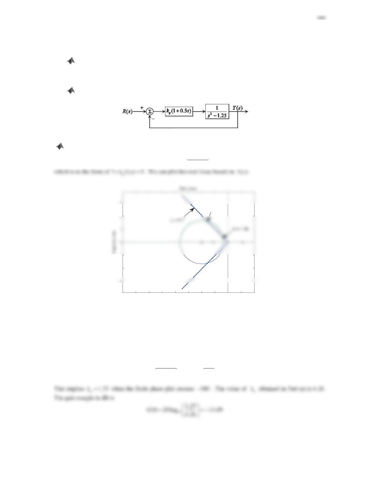
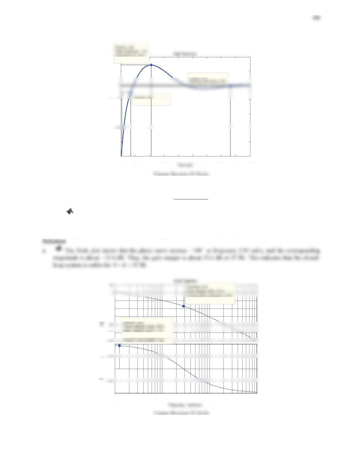
6. Consider the unity negative feedback system with a PD controller as shown in Figure 10.91.
a. Determine the value of the proportional gain kpsuch that the damping ratio of the closed-loop system
is 0.7.
b. What is the GM of the system if kpis set to the value obtained in Part (a)? Answer this question without
creating the Bode plots.
c. Verify your answer in Part (b) by creating the Bode plots using MATLAB.
Figure 10.91 Problem 6.
Solution
a. The characteristic equation of the closed-loop system is
p2
1
1 1 0.5 0
1.25
ks
s
Real Axis
-8 -7 -6 -5 -4 -3 -2 -1 01 2
-2
-1
K = 6.26
Figure Review10 No6a
As shown in the root locus, the dashed diagonal lines indicate pole locations with a damping ratio of 0.7. When
1.56
p
k
or 6.26, the damping ratio of the closed-loop system is 0.7. Choose
p
6.26k
.
b. The root locus crosses the imaginary jZ-axis at 0s . Thus, we have
pp
2
1 0.5 1
110
1.25 1.25
s
kk
s
§·
¨¸
©¹
491
c. The Bode plot of
p
()kLs
when
p
6.26k
is shown below. The gain margin and phase margin are
14
dB
and
58.7
D
. Note that based on the root locus, the stability of the closed-loop system changes from unstable to
stable instead of from stable to unstable when the gain
p
k
increases. The gain margin and phase margin give the
conflict conclusions on stability (
GM 0
dB and
PM 0!
D
.)
Bode Diagram
-180
-135
Phase Margin (deg): 58.7
Delay Margin (sec): 0.312
At frequency (rad/sec): 3.28
Closed Loop Stable? Yes
Phase (deg)
-20
0
10
20
System: untitled1
Gain Margin (dB): -14
At frequency (rad/sec): 0
Magnitude (dB)
7. Consider the system
>@
11 1
22 2
01 0
,10.
23 1
xx x
uy
xx x
½ ½ ½
ªºªº
®¾ ®¾ ®¾
«»«»
¬¼¬¼
¯¯ ¯
¿¿ ¿
a. Design a state-feedback controller so that the closed-loop unit-step response has an overshoot of less than
5% and a peak time under 1.5 s.
b. Verify your result in Part (a) with MATLAB.
Solution
a. For the given system,
11
22
01 0
23 1
xx
u
xx
½ ½
ªºªº
®¾ ®¾
«»«»
¯¿¬ ¼¯¿¬¼
,
>@
1
2
10 x
yx
½
®¾
¯¿
492
b. The following MATLAB command session returns
>@
7 1.2 K
.
A = [0 1; -2 -3];
B = [0; 1];
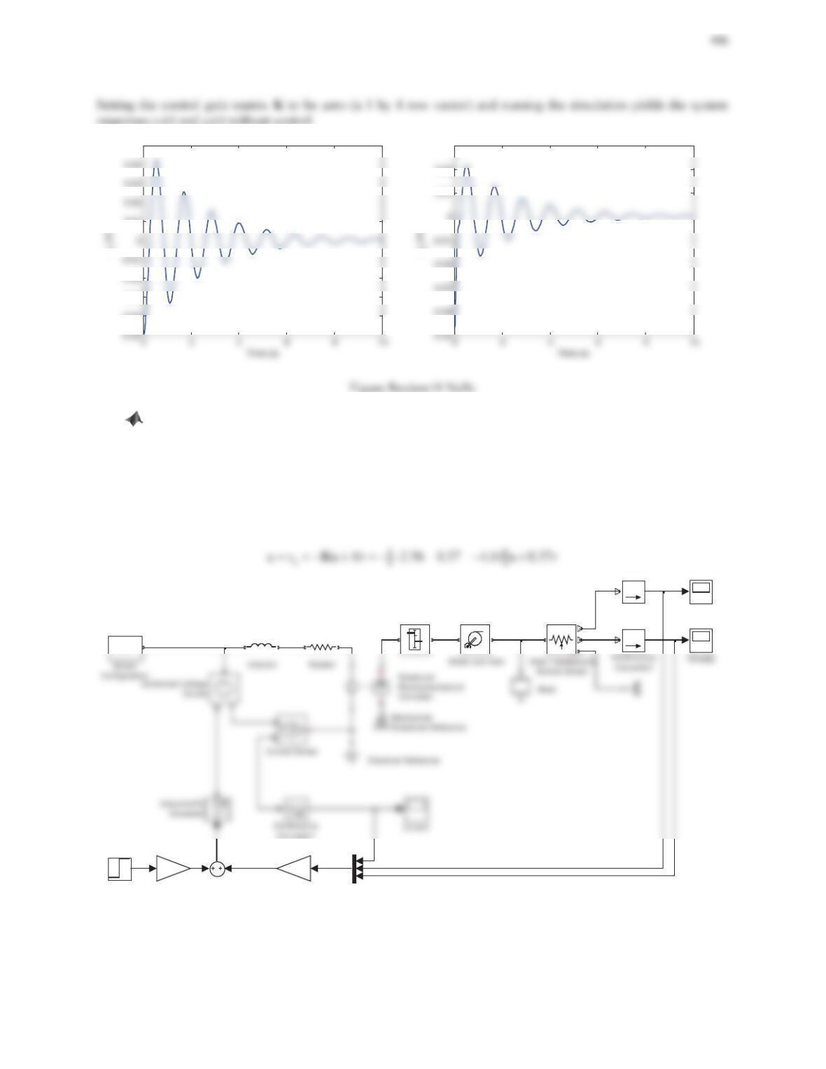
8. Consider the cart–inverted-pendulum system shown in Figure 5.79. Assume that the mass of the cart is 0.8
kg, the mass of the pendulum is 0.2 kg, and the length of the pendulum is 0.6 m.
a. Determine the poles of the linearized system. Is it stable or unstable?
b. Design a full-state feedback controller such that the closed-loop poles are located at
1,2
2.90 2.15jp r
,
3
10p
, and 420p .
c. Assume that the initial angle of the inverted pendulum is 5° away from the vertical reference line. Using the
state feedback gain matrix Kobtained in Part (b), examine the responses of the nonlinear and linearized
closed-loop systems using Simulink.
Solution
a. The state-space model of the cart-inverted-pendulum system in Figure 5.79 is
11 1
0010 0
0001 0
xx x
ªºªº
«»«»
½ ½ ½
The following MATLAB session returns the open-loop poles, which are 0, 0, and 5.37r. The system is
unstable.
% system parameters
M = 0.2; % mass of the pendulum
g = 9.81;
% state space matrices
A = [0 0 1 0;
0 0 0 1;
>@
90.34 177.54 53.75 33.67 K
c. The Simulink block diagrams and the responses of the cart and the pendulum are shown below.
x
1
s
Integrator
C* u
C
B* u
B
Figure Review10 No8a
To construct the Simulink block diagram for nonlinear simulation, substituting the parameter values into the
nonlinear model,
2
11
() cos sin
22
mMx ML ML f
TTTT
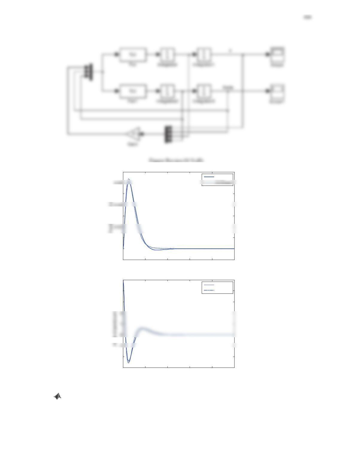
0 1 2 3 4 5
-0.01
0
0.01
0.03
0.05
0.07
Time (s)
linear
0 1 2 3 4 5
-3
-2
3
4
5
Time (s)
linear
nonlinear
Figure Review10 No8c
9. Consider the two-degree-of-freedom quarter-car model shown in Figure 5.34, where the force f, applied
between the car body and the wheel–tire–axle assembly, is controlled by feedback and represent the active
495
components of the suspension system. Assume that 1212
20568 30493 1278 3189fxxxx
. Build a
Simulink block diagram of the feedback control system. Find the displacement responses x1(t) and x2(t) if
initially x1=0.05 m and x2=0.05m. Ignore the displacement input z(t). What are the system responses x1(t)
and x2(t) without control?
Solution
The Simulink block diagram is shown below, where the quarter-car model is represented in the state-space form,
0010 0
xxx
ªºªº
«»«»
½ ½ ½
Figure Review10 No9a
The displacement responses x1(t) and x2(t) for initial values of x1=0.05 m and x2=0.05m are shown below.
0246810
-0.06
Time (s)
0246810
-0.05
-0.01
0.01
Time (s)
Figure Review10 No9b
-0.04
-0.03
0.01
0.05
x
0.02
0.03
x
10. Consider the DC motor driven wheeled mobile robot shown in Figure 6.83, where the voltage applied to
the DC motor is computed by a controller. Assume that
a
2.56 0.37 4.61 0.37vixxr
, where ris a
reference trajectory that the cart should follow. Build a block diagram of the feedback control system, where the
mobile robot is constructed using Simscape blocks and the controller is constructed using Simulink blocks. Find
the displacement response x(t) of the mobile robot if a unit-step reference command signal is sent to the system.
Solution
The Simulink block diagram is shown below, where the controller is
PA
Step
refe rence
f(x)=0
–+
SPS
SPS
PS-Simulink
Converter
0.37
N
–+
P
V
R
OS
Gear Box
Displ acement
K*u
-K
Figure Review10 No10a
00.2 0.4 0.6 0.8 1
0
0.2
0.6
1
1.2
Time (s)
Figure Review10 No10b