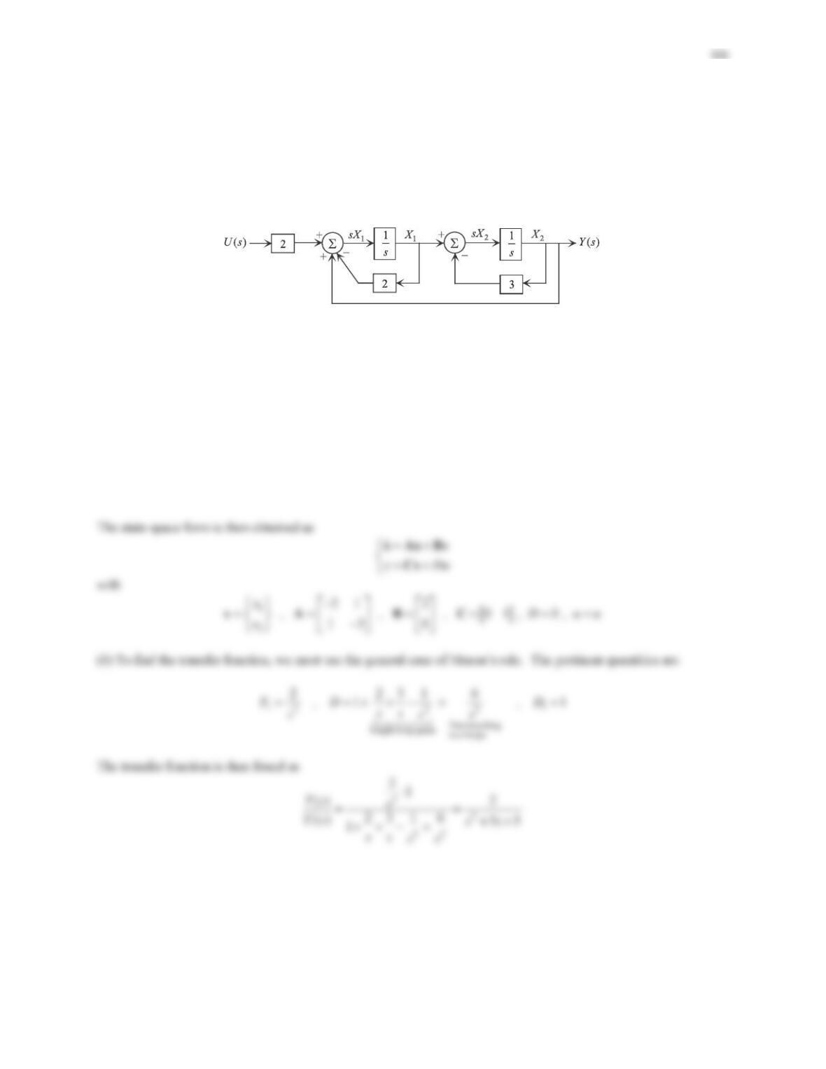
20. The block diagram representation of a system model is presented in Figure 4.33, where U,
1
X
,2
X
, and
Y
denote the Laplace transforms of the input, the two state variables, and the output.
(a) Derive the state-space form directly from the block diagram.
(b) Find the transfer function directly from the block diagram.
Figure 4.33 Problem 20.
Solution
(a) We first find
12 1
2
21 2
22
,
3
sX X X U YX
sX X X
®
¯
Consequently, the state-variable equations and the output equation are derived as
12 1
2
21 2
22
,
3
xx x u yx
xx x
®
¯
Problem Set 4.6
In Problems 1–10, the mathematical model of a nonlinear dynamic system is given. Follow the procedure outlined
in this section to derive the linearized model.
1.
3
2 1 sin 2 , (0) 0 , (0) 1xxx t x x
106
Solution
The 4-step procedure is followed as listed below:
Step 1: The operating point satisfies
3
1x
so that
1x
.
Step 2: The nonlinearity
3
()fx x
is linearized about
1x
as
32
1
() (1) 3 1 3
x
fx x f x x x
ªº
# ‘ ‘
¬¼
2.
2 2 cos , (0) 0 , (0) 1xx xx t x x
Solution
The 4-step procedure is followed as listed below:
Step 1: The operating point satisfies
22xx
so that
1x
.
Step 2: The nonlinearity
()fx xx
is linearized about
1x
as
3.
2 2 sin , (0) 0 , (0) 1xx xx t x x
Solution
We follow the 4-step procedure outlined in the section. First note that
2Differentiate
2
2 if 0 4 if 0
( ) 2 ( ) 4 if 0
2 if 0
xx xx
fx xx f x xx
xx
tt
°c
®®
¯
°
¯
107
4.
1 sin , (0) 1 , (0) 0xxxx t x x
Solution
First note that
3
2
3
2
if 0
if 0
( ) ( ) if 0
if 0
xx
xx x
fx x x f x
xx
xx x
t
t
°°
c
®®
°°
¯¯
108
5.
1
4
2 if 0
( ) 1 cos , (0) , (0) 1 , ( )
2 if 0
xx
xx fx t x x fx
xx
t
°
®d
°
¯
Solution
Step 1: The operating point satisfies
() 1fx
.
6.
12 1
3
2
21112
(0) 1
, (0) 1
2sin
xx x
x
xxxxx t
°
®
°
¯
Solution
Step 1: The operating point
12
,xx
satisfies
109
7.
3 ( ) 3 cos , (0) 1 , (0) 0xxgx t x x
,
3(1 ) if 0
()
3(1 ) if 0
x
x
ex
gx
ex
t
°
®
°
¯
Solution
Step 1: The operating point
x
satisfies
() 3gx
. Due to the nature of
()gx
, we need to inspect two cases:
8.
121 1
12
22
(0) 0
, (0) 1
21
xxx x
x
xx t
°
®
°
¯
Solution
Step 1: The operating point satisfies
21 2
11
2
02
Operating point : ( 2, 2)
2
210
xx x
x
x
°
®
°
¯
110
Step 2: Linearize
1
22
()2fx x
about the operating point:
9.
31
112
2
21
(0) 1
3 , (0) 0
24 sin
x
xxx
x
xx t
°
®
°
¯
Solution
Step 1: The operating point satisfies
32
21
1
1
2
30
24
24 0
x
xx
x
x
°
®
°
¯
111
10.1
1211
2
212
(0) 1
2 cos 3 , (0) 2
2
x
xxxx t
x
xxx
°
®
°
¯
Solution
Step 1: The operating point
12
(, )xx
satisfies
In Problems 11–14, a nonlinear model is provided.
(a) Obtain the linear state-space form using MATLAB Simulink,
(b) Derive the linearized model analytically to confirm the findings in Part (a).
11.
3
2 1 sin 2 , (0) 0 , (0) 1xxx t x x
Solution
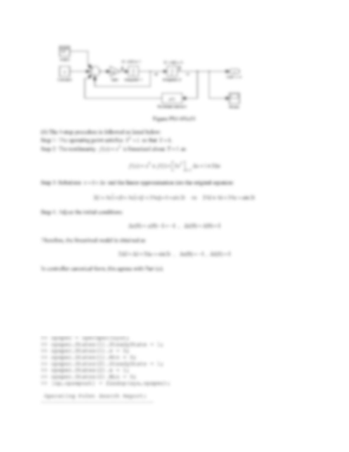
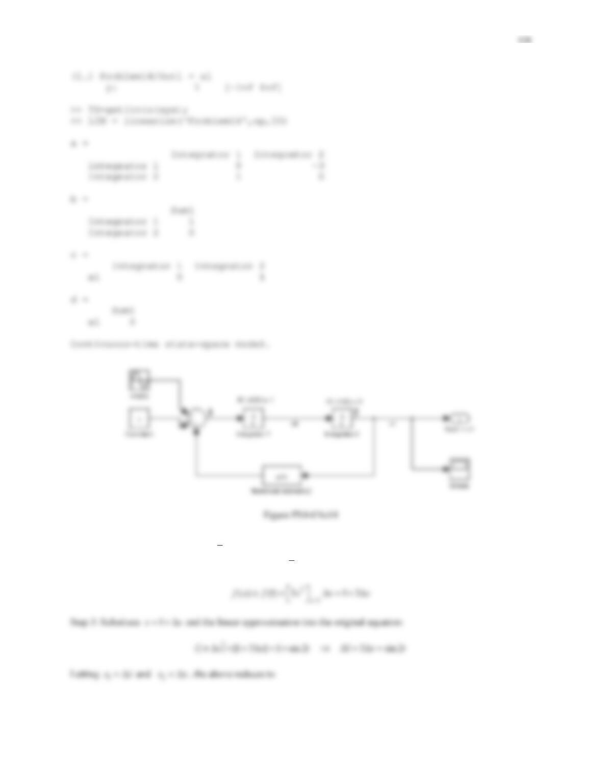
(a) The Simulink model is built as shown in Figure PS4-6No11 and saved as ‘Problem11‘. Employing the
procedure outlined in this section, we find the operating point and the state-space model as follows.
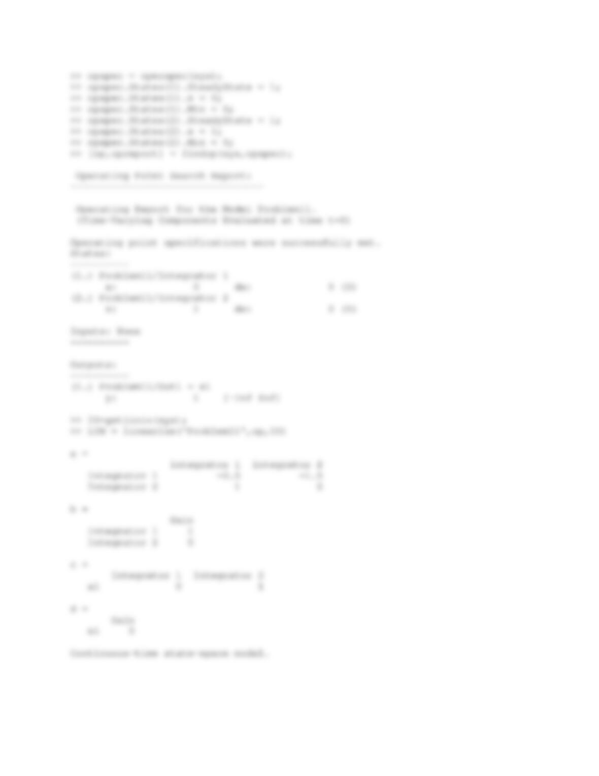
>> sys=’Problem11′;
>> load_system(sys);
112
113
12.
3
2 sin , (0) 0 , (0) 1xx x t x x
Solution
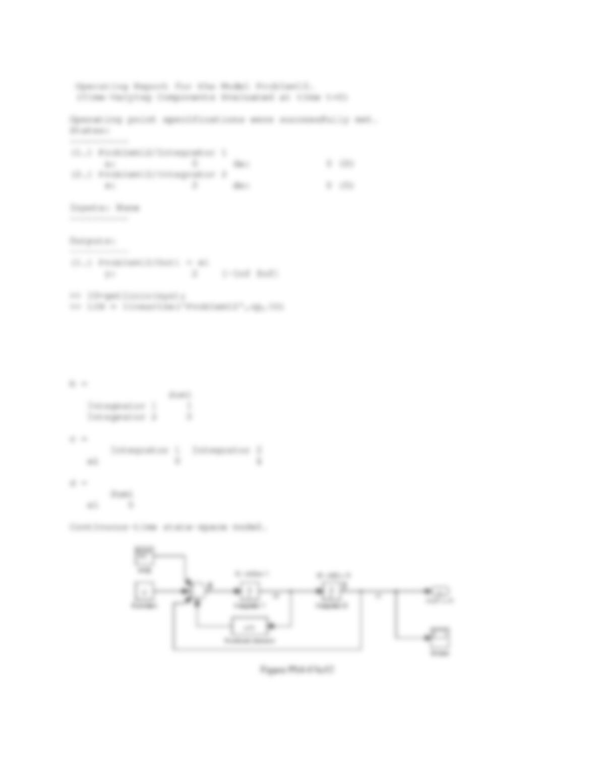
(a) The Simulink model is built as shown in Figure PS4-6No12 and saved as ‘Problem12‘. Employing the
procedure outlined in this section, we find the operating point and the state-space model as follows.
>> sys=’Problem12′;
>> load_system(sys);
114
a =
Integrator 1 Integrator 2
Integrator 1 -1e-010 -1
Integrator 2 1 0
115
13.
1 cos 2 , (0) 0 , (0) 1xxx x t x x
Solution
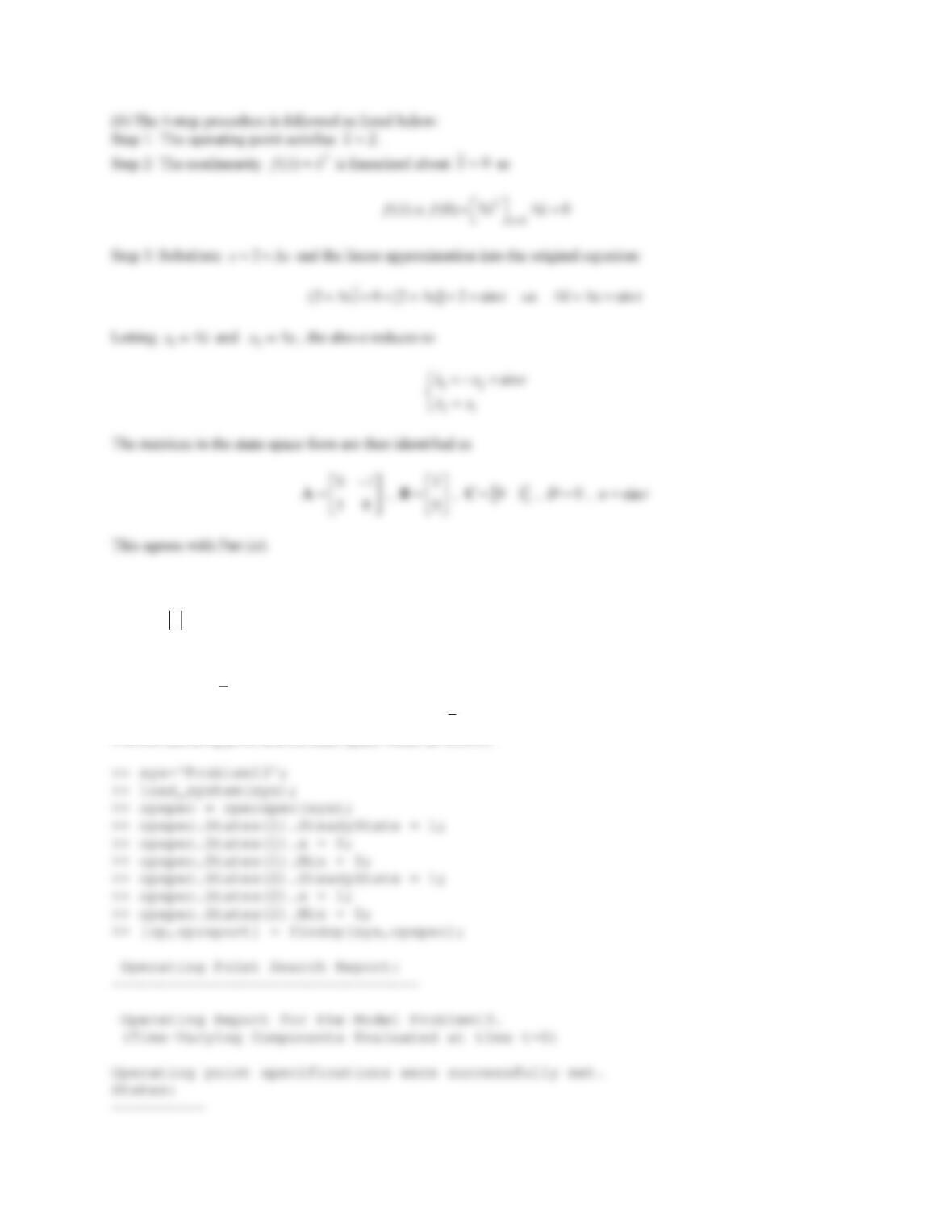
(a) The Simulink model is built as shown in Figure PS4-6No13 and saved as ‘Problem13‘. Noting that
1
2
cos 2 sin 2tt
S
, we generate cos 2tusing the Sine Wave block from the Sources library by setting the
amplitude to
1
, frequency to
2 rad/sec
, and phase to
1
2
S
. Employing the procedure outlined in this section, we
find the operating point and the state-space model as follows.
(1.) Problem13/Integrator 1
x: 0 dx: 0 (0)
(2.) Problem13/Integrator 2
x: 2 dx: 0 (0)
117
This agrees with Part (a).
14.
3
1 sin 2 , (0) 0 , (0) 1
xx t x x
Solution
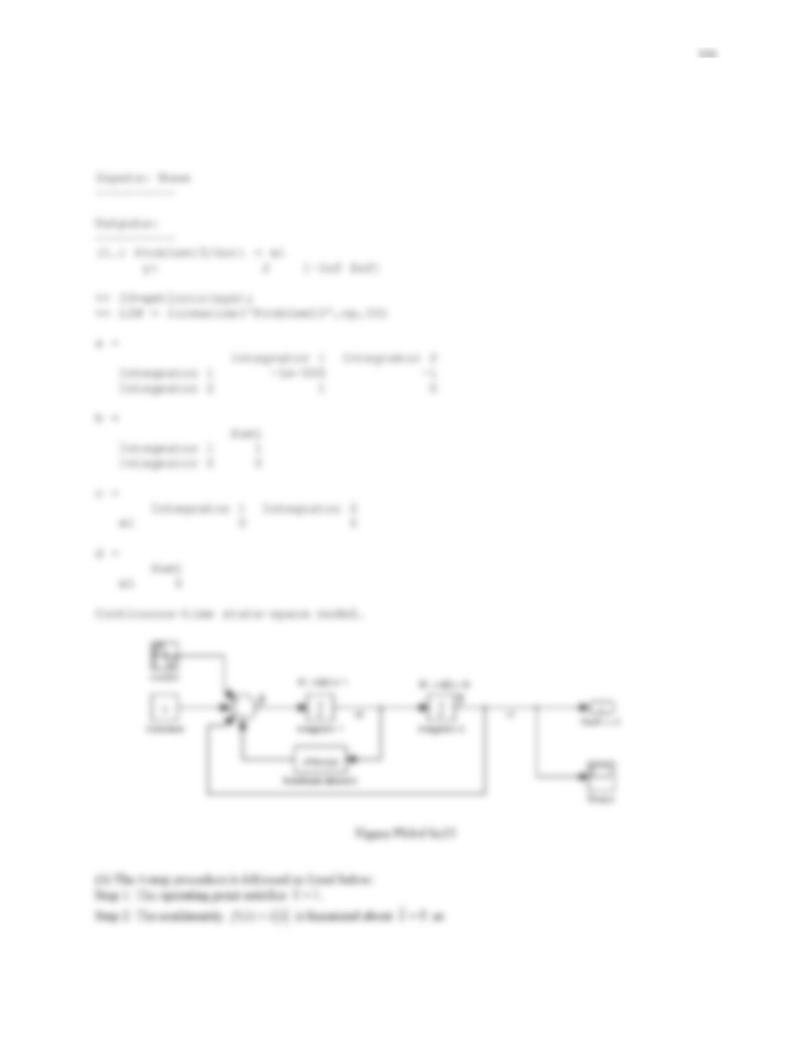
(a) The Simulink model is built as shown in Figure PS4-6No14 and saved as ‘Problem14‘. Employing the
procedure outlined in this section, we find the operating point and the state-space model as follows.
>> sys=’Problem14′;
>> load_system(sys);
>> opspec = operspec(sys);
>> opspec.States(1).SteadyState = 1;
>> opspec.States(1).x = 0;
———-
(b) The 4-step procedure is followed as listed below:
Step 1: The operating point satisfies
1x
.
Step 2: The nonlinearity
3
()fx x
is linearized about
1x
as
119
Review Problems
1. The governing equations for a dynamic system are given as
111 2
21 2
23()
3 2 0
xxx x ft
xx x
®
¯
(a)Assuming ()ft and
1
x
are the input and output, respectively, obtain the state-space form.
(b) Determine whether the system is stable.
(c) Find the transfer function directly from the governing equations.
Solution
(a) There are three state variables: 11
xx ,
22
xx
,31
xx . The state-variable equations are
>@
13
1
212
3
1
2
3
xx
xxx
xxxxf
°
°
®
°
ªº