Archives
Chapter 1 Homework The digits to the left of the decimal point are treated exactly
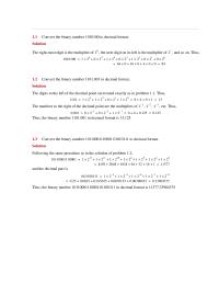
1.1 Convert the binary number 1010100 to decimal format. Solution 1.2 Convert the binary number 1101.001 to decimal format. Solution The digits to the left of the decimal point are treated exactly as in problem 1.1. Thus, The numbers to […]
Chapter 1 Homework The Largest Number That Could Converted With
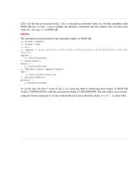
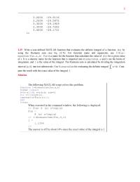
1.23 Use the first seven terms in Eq. (1.21) to calculate an estimated value of e. Do the calculation with MATLAB (use format long to display the numbers). Determine the true relative error. For the exact value of e, use […]
Chapter 1 Homework The largest numbers that could be added with the function
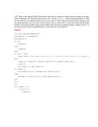
1.37 Write a user-defined MATLAB function that adds two integers in binary form according to the algo- rithm of Problem 1.30. Name the function aplusb = addbin(a,b), where the input arguments a and b are the numbers to be added […]
Chapter 10 Homework Output Variable Vector With The Coordinate The
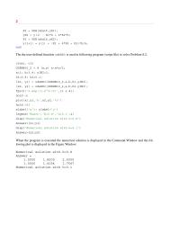
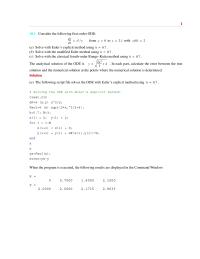
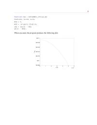
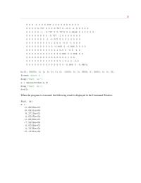
2 The the user-defined function odeRK3 is used in following program (script file) to solve Problem 8.2. clear, clc ODEHW10_2 = @ (x,y) x-x*y/2; a=1; b=3.4; yINI=1; h1=0.8; h2=0.1; [x1, y1] = odeRK3(ODEHW10_2,a,b,h1,yINI); [x2, y2] = odeRK3(ODEHW10_2,a,b,h2,yINI); fplot(‘2-exp((1-x^2)/4)’,[1 3.4]) hold […]
Chapter 10 Homework Problem Part A Solving The Ode
1 10.1 Consider the following first-order ODE: from to with (a) Solve with Euler’s explicit method using . (b) Solve with the modified Euler method using . (c) Solve with the classical fourth-order Runge–Kutta method using . The analytical solution […]
Chapter 10 Homework The Program Should Also Plot The Exact
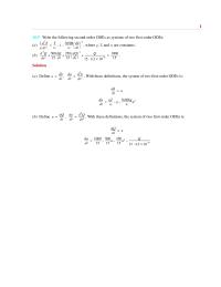
1 10.9 Write the following second-order ODEs as systems of two first-order ODEs: (a), where g, T, and w are constants. (b). Solution (a) Define , . With these definitions, the system of two first-order ODEs is: 1 g —–d2h […]
Chapter 10 Homework When The Script File Executed The Following
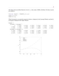
3 The listing of the user-defined function ODEsHW10_6 (the system of ODEs in Problem 10.6) that is used in the solution is: When the program is executed the numerical solution is displayed in the Command Window and the fol- lowing […]
Chapter 11 Homework A vector with the x coordinate of the solution points
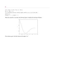
4 a=0; b=pi; n=100; Ya=1.5; Yb=0; WL=-5; WH=-1.5; When the script file is executed, the following figure is displayed in the Figure Window: This solution agrees with the solution in Example 11-6. 00.5 11.5 22.5 3 3.5 −1 −0.5 0 […]
Chapter 11 Homework difference formula for approximating the second derivative
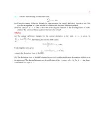
1 11.1 Consider the following second-order ODE: (a) Using the central difference formula for approximating the second derivative, discretize the ODE (rewrite the equation in a form suitable for solution with the finite difference method). (b) If the step size […]
Chapter 11 Homework The axial temperature variation of a current-carrying bare wire
3 function res = bcfunHW11_27b(ya,yb) Tinf=300; h=100; k=72; When executed, the program produces the following plot: 0123456 x 10-5 624.098 624.1 624.102 624.104 x (m) T (K) 624.106 624.108 624.11 BCa = 0; BCb = -h*(yb(1)-Tinf)/k; res = [ya(2) – […]
Chapter 11 Homework Use Second order Accurate Central Differences For All
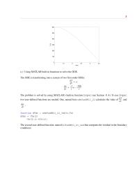
3 (c) Using MATLAB built-in functions to solve the ODE. The ODE is transforming into a system of two first-order ODEs: 0 100 200 300 400 T (C) 11.5 22.5 33.5 500 600 r (cm) dT dr —–– w= dw […]
Chapter 2 Homework by the intermediate value theorem, there exists at least one
1 ______________________________________________________________________________ (2.1) Apply the intermediate value theorem to show that the polynomial 24x10x)x(f 2−+−= has a root in the interval [3,5]. Solution The intermediate value theorem (see Section 2.2) guarantees that there exists at least one 2.2 Apply the […]
Chapter 2 Homework How much rope should be used for the square and how much for
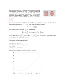
2.36 Rope with a length of 10 m is to be used to enclose a square area with side x and a circular area with radius r. How much rope should be used for the square and how much for […]
Chapter 2 Homework The Two Matrices And Must Supplied The
2 ______________________________________________________________________________ 2.25 Write a user-defined MATLAB function that evaluates the definite integral of a function by using the Riemann sum (see Eq. (2.7)). For function name and arguments, use I=Rie- mannSum(Fun,a,b). Fun is a name for the function that […]
Chapter 3 Homework Determine The Angle For Which First Derive
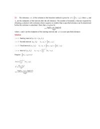
3.1 The tolerance, , of the solution in the bisection method is given by , where and are the endpoints of the interval after the nth iteration. The number of iterations n that are required for obtaining a solution with […]
Chapter 3 Homework For Nickel Which Sometimes Used Such Detectors
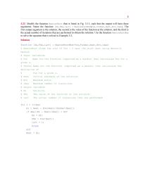
1 3.23 Modify the function NewtonRoot that is listed in Fig. 3-11, such that the output will have three arguments. Name the function [ Xs,FXs,iact] = NewtonRootMod ( Fun,FunDer,Xest,Err,imax ) . The first output argument is the solution, the second […]
Chapter 3 Homework Solution Function Square root p Square root Finds The Root
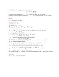
3.14 Solve the following system of nonlinear equations: (a) Use Newton’s method. Start at , , and carry out the first five iterations . (b) Use the fixed-point iteration method. Start at , , and carry out the first five […]
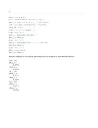
Chapter 3 Homework This Iteration Function Used The Following Mat lab
2 Con=w/(360*L*E*I); y=@(x) Con*x*(7*L^4-10*L^2*x^2+3*x^4); yd=@ (x) Con*(7*L^4-10*L^2*3*x^2+3*5*x^4); ydd=@ (x) Con*(-10*L^2*3*2*x+3*5*4*x^3); When the script file is executed the following results are displayed in the Command Window: Part (a) xMax_a = 2.0773 yMax_a = 0.0090 Part (b) xMax_b = 2.0773 yMax_b = […]
Chapter 4 Homework Carry out the first three iterations of the solution
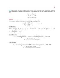
1 4.15 Carry out the first three iterations of the solution of the following system of equations using the Gauss–Seidel iterative method. For the first guess of the solution, take the value of all the unknowns to be zero. Solution […]
Chapter 4 Homework The Pivot Element Now Use The Second
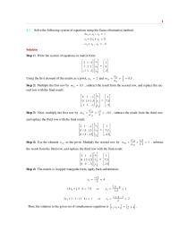
1 4.1 Solve the following system of equations using the Gauss elimination method: Solution Step 1: Write the system of equations in matrix form: Using the first element of the matrix as a pivot, and . 2x1x2x3 –+1= x12x2x3 ++ […]
Chapter 4 Homework The problem is solved by solving the following system
3 0 0 0 -1 0 0 0.707 1 0 0 0 0 0 0 0 0 0 0 0 0 0 0.707 0 0 0 0.707 0 -0.5 -1 0 0 0 0 0 0 0 0 0 0 […]
Chapter 4 Homework The user-defined function is used in the Command Window
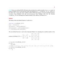
1 4.28 Write a user-defined MATLAB function that calculates the condition number of an matrix by using the infinity norm. For the function name and arguments use c = CondNumb_Inf(A), where A is the matrix and c is the value […]
Chapter 5 Homework Show that the eigenvalues of the following matrix
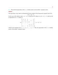
1 5.1 Show that the eigenvalues of the identity matrix are the number 1 repeated n times. Solution The eigenvalues of any matrix are determined from the solution of the characteristic equation, Eq.(4.93): nn× det a λI–[]0= For the case […]
Chapter 5 Homework These Two Equations Can Solved For And
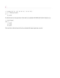
2 >> sigma=[40 20 -18; 20 28 12; -18 12 14]; >> e = MaxEig(Sigma) e = 56.4898 To check the answer, the eigenvalues of the matrix are calculated with MATLAB’s built-in function eig: >> eig(Sigma) ans = -7.2389 32.7493 […]
Chapter 6 Homework it is only necessary to calculate the linear spline between
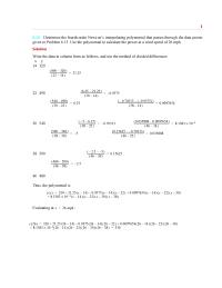
1 6.14 Determine the fourth-order Newt on’s interpolating polynomial that passes through the data poi nts given in Problem 6.13. Use the polynomial to calculate the power at a wind speed of 26 mph. Solution Write the data in column […]
Chapter 6 Homework Determine The Coefficients The Exponential
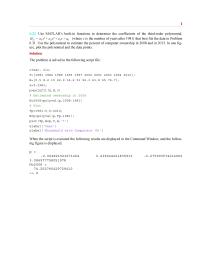
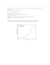
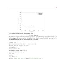
1 6.32 Use MATLAB’s built-in functions to determine the coefficients of the third-order polynomial, (where x is the number of years after 1981) that best fits the data in Problem 6.31. Use the polynomial to estimate the percent of computer […]
Chapter 6 Homework Once And Are Calculated And Are Determined
3 y=[0 3 4.5 5.8 5.9 5.8 6.2 7.4 9.6 15.6 20.7 26.7 31.1 35.6 39.3 41.5]; n=length(x); [a,Er] = CubicPolyFit(x,y) When the program is executed, the following plot is displayed in the Figure Window: 0 1 2 3 4 […]
Chapter 6 Homework The Computer Program Calculates The Constants And
3 (b) Quadratic function that fits the data has the form: The following program written in a script file uses the user-defined function QuadFit from Problem 5.20 to find the quadratic function that best fits the data. It also plots […]
Chapter 6 Homework The Following Data Give The Approximate Population
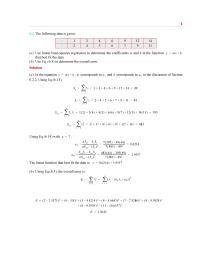
1 6.1 The following data is given: (a) Use linear least-squares regression to determine the coefficients m and b in the functi on that best fit the data. (b) Use Eq. (6.5) to determine the overall error. Solution (a) In […]
Chapter 8 Homework slope and the two-point central difference formula applied
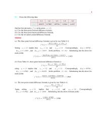
1 8.1 Given the following data: find the first derivative at the point . (a) Use the three-point forward difference formula. (b) Use the three-point backward difference formula. (c) Use the two-point central difference formula. Solution (a) The three point […]
Chapter 8 Homework the following results are displayed in the Command Window
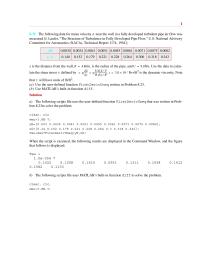
1 8.35 The following data for mean velocity near the wall in a fully developed turbulent pipe air flow was measured [J. Laufer, “The Structure of Turbulence in Fully Developed Pipe Flow,” U.S. National Advisory Committee for Aeronautics (NACA), Technical […]
Chapter 8 Homework The output arguments dfdx2 and dfdy2 are vectors with the
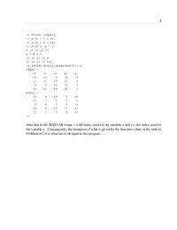
3 >> format compact >> x=[0 1 2 3 4]; >> y=[0 1 2 3 4]; >> f=[0 3 14 7 5 8 10 14 12 10 2 7 8 9 7 Note that in the MATLAB script, i is […]
Chapter 8 Homework Use Lagrange Polynomials Develop Difference Formula
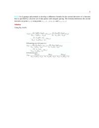
1 8.15 Use Lagrange polynomials to develop a difference formula for the second derivative of a function that is specified by a discrete set of data points with unequal spacing. The formula determines the second derivative at point using points […]
Chapter 9 Homework Determine The Volume The Silo Problem
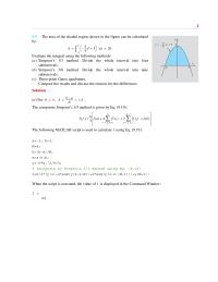
1 9.9 The area of the shaded region shown in the figure can be calculated by: Evaluate the integral using the following methods: (a) Simpson’s 1/3 method. Divide the whole interval into four subintervals. (b) Simpson’s 3/8 method. Divide the […]
Chapter 9 Homework the subintervals are all the same width
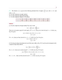
1 9.1 The function is given in the following tabulated form. Compute with and with . (a) Use the composite rectangle method. (b) Use the composite trapezoidal method. (c) Use the composite Simpson’s 3/8 method. Solution (a) For the composite […]