Chapter 11 Homework difference formula for approximating the second derivative

1

11.1 Consider the following second-order ODE:

(a) Using the central difference formula for approximating the second derivative, discretize the ODE

(rewrite the equation in a form suitable for solution with the finite difference method).

(b) If the step size is , what is the value of the diagonal elements in the resulting matrix of coeffi-

cients of the system of linear equations that has to be solved?

Solution

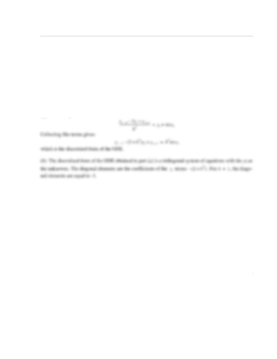
(a) The central difference formula for the second derivative at the point is given by

. Substituting this into the ODE yields:

d2y

dx2

——––yxsin+=

h1=

xx

i

=

d2y

dx2

——-–yi1– 2yi

–yi1+

+

h2

—————–———————-–

=

1

11.2 Consider the following second-order ODE:

where C is a constant.

(a) Using the central difference formula for approximating the second derivative, discretize the ODE

(rewrite the equation in a form suitable for solution with the finite difference method).

(b) If the step size is , what is the value of the diagonal elements in the resulting matrix of coeffi-

cients of the system of linear equations that has to be solved?

Solution

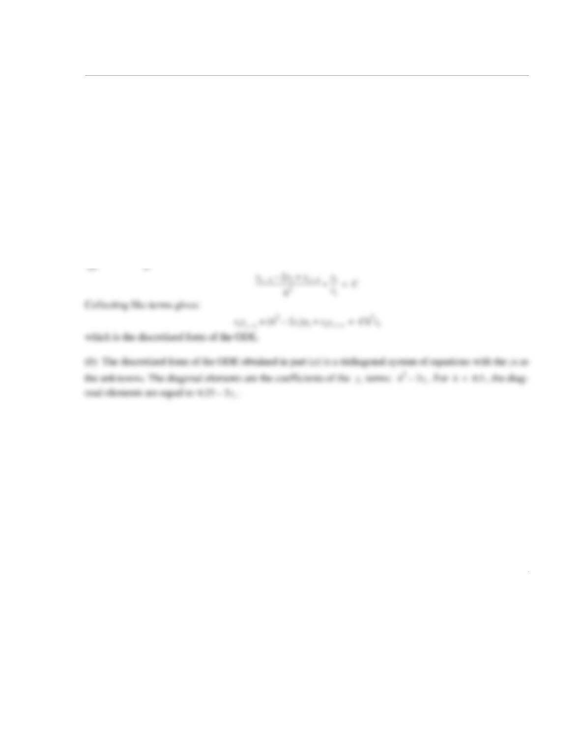
(a) The central difference formula for the second derivative at the point is given by

. Substituting this into the ODE yields:

d2y

dr2

——––y

r

—

+C=

h0.5=

xx

i

=

d2y

——-–yi1– 2yi

–yi1+

+

—————–———————-–

=

1

11.4 Consider the following boundary value problem:

for , with the boundary conditions: and

where a and b are constants. Discretize the second-order ODE using:

(a) Second-order accurate forward difference.

(b) Second-order accurate backward difference.

(c) Discretize the boundary condition at using the second-order accurate forward difference.

Solution

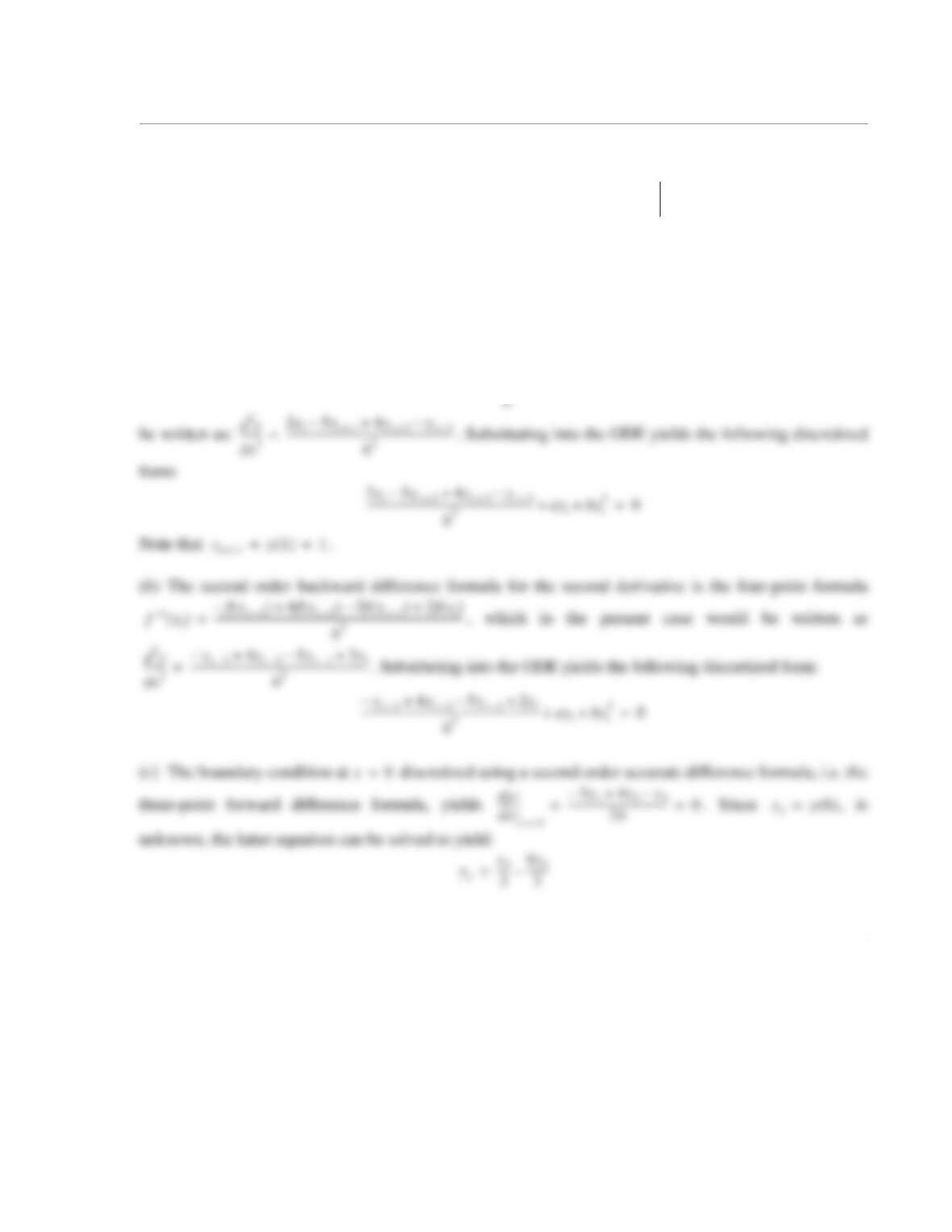
(a) The second-order accurate forward difference formula for the second derivative is the four-point for–

mula given in Table 6-1, , which in the present case would

d2y

dx2

——––ay by4

++ 0=

0x1≤≤

dy

dx

—––

x0=

0=

y1() 1=

x0=

f′′ xi

() 2fx

i

() 5fx

i1+

()–4fx

i2+

()fx

i3+

()–+

—————–———————————-———————————-——

=

1

11.7 Consider the following boundary value problem:

for , with the boundary conditions: and

What are the diagonal elements of the resulting tridiagonal matrix when the finite difference method with

first-order accurate central differences is applied to solve the problem with a step size of 1/4?

Solution

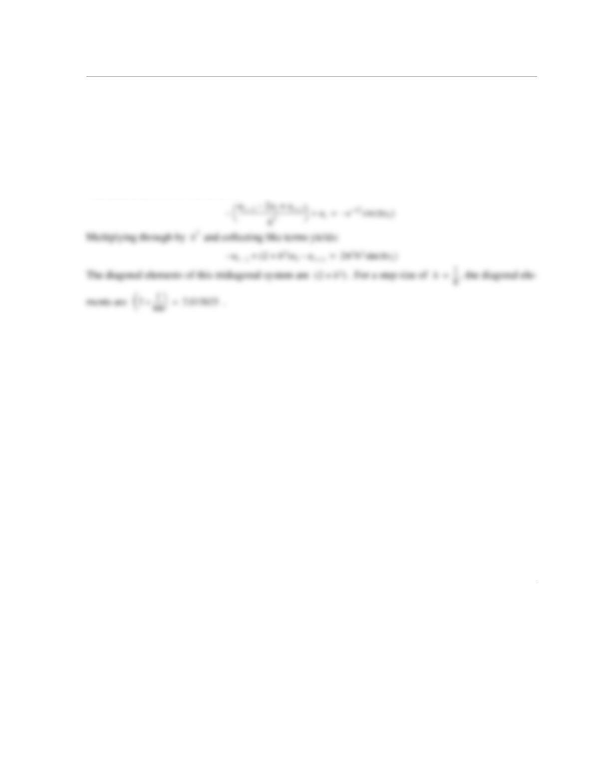
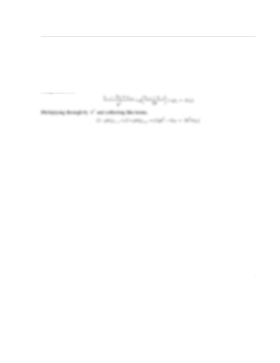
The discretized form of the ODE is:

d2u

dx2

——––u–ex2

–πx()sin–=

0x1≤≤

u0() 1=

u1() 1–=

1

11.8 Consider the second-order ODE of the form:

where p and q are constants, and is a given function. Using second-order accurate central differences

for the derivatives, discretize the ODE.

Solution

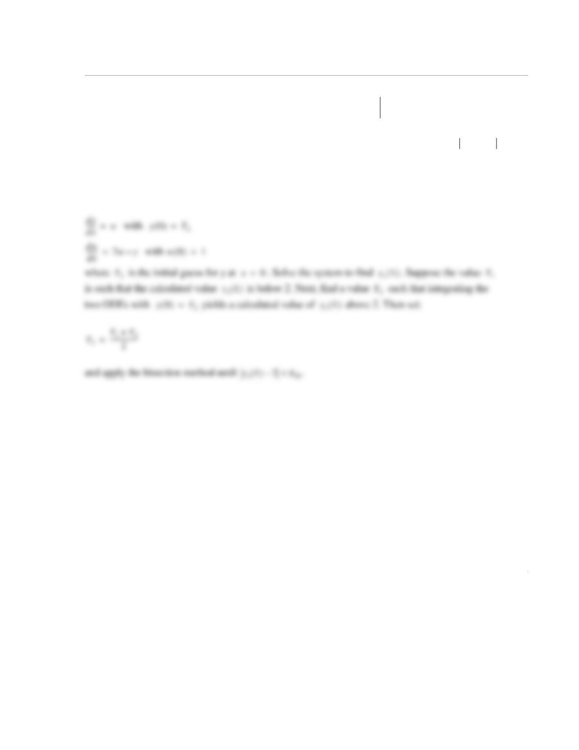
Using Table 6-1,

d2y

dx2

——––pdy

dx

—––qy++ rx()=

rx()

1

11.9 Given the boundary value problem , with and . Set up the

problem for solving using the shooting method. Use the bisection method to determine the value of

such that the boundary condition at is met within a specified error defined as where

is the calculated value of the solution at . Set up the equations to be solved but do not solve.

Solution

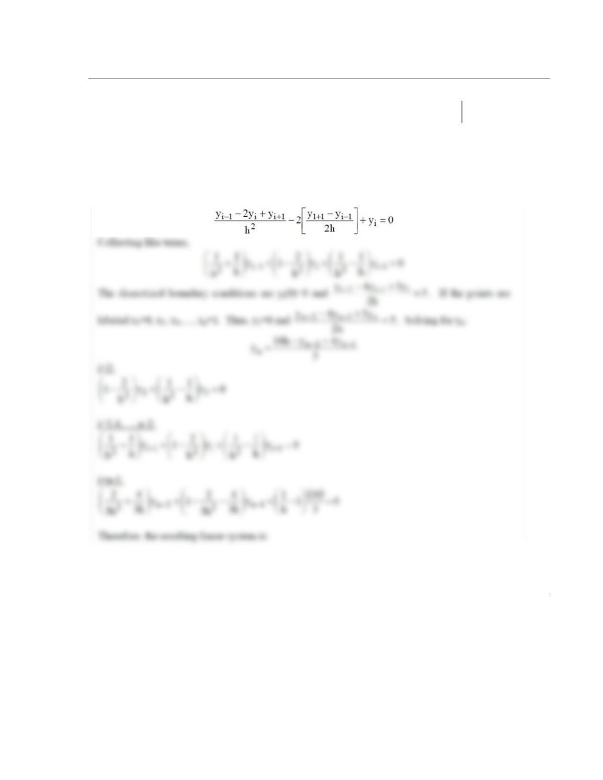
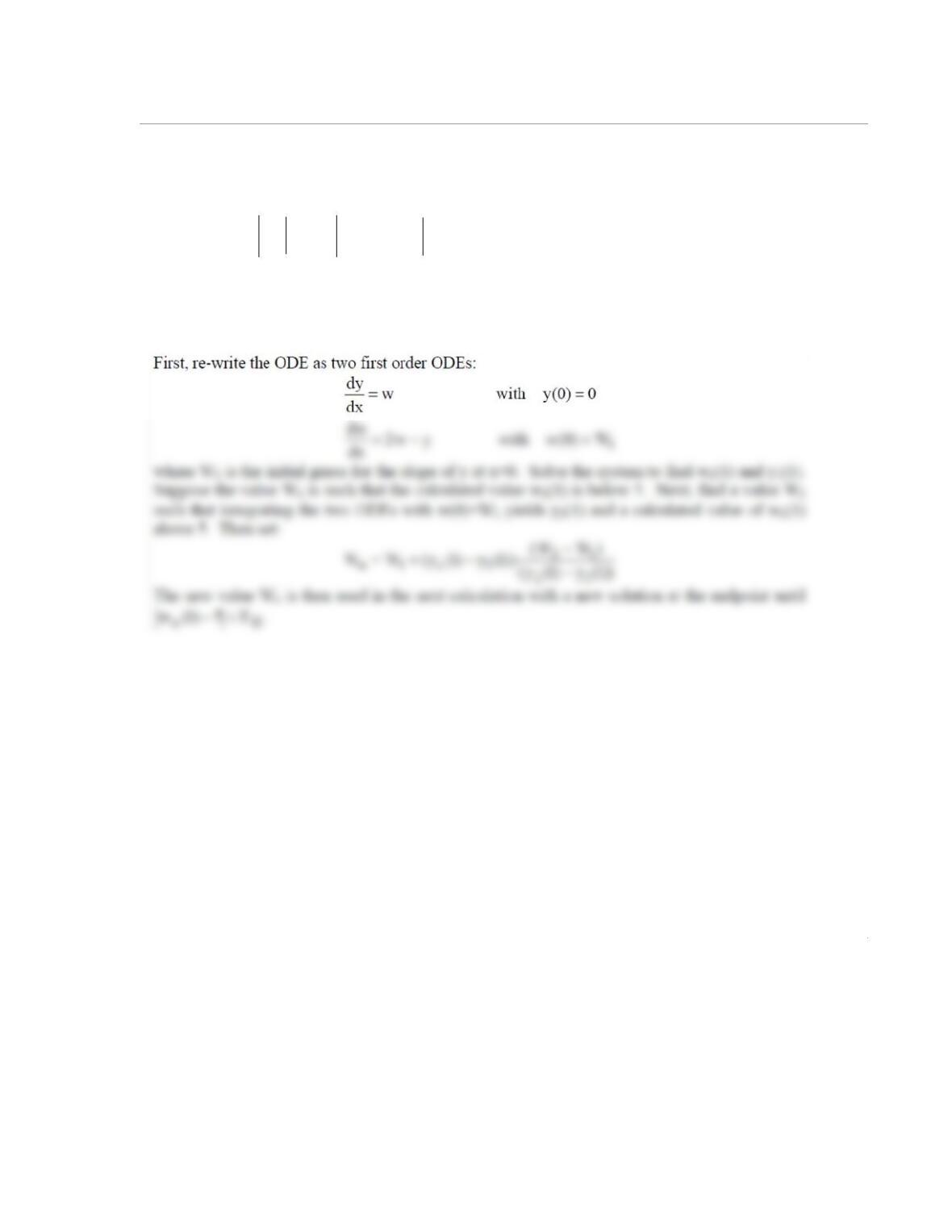
First, re-write the ODE as two first order ODEs:

d2y

dx2

——––2dy

dx

—––

–y+0=

dy

dx

—––

x0=

1=

y1() 2=

y0()

x1=

EHyc1() 1–=

yc1()

x1=

1

11.10 Given the boundary value problem , with and . Discretize

the problem using second-order accurate central differences for the derivatives and a second-order accurate

one-sided difference for the boundary condition at . For a constant step size h, what is the term on

the right-hand side of the last of the simultaneous equations that result?

Solution

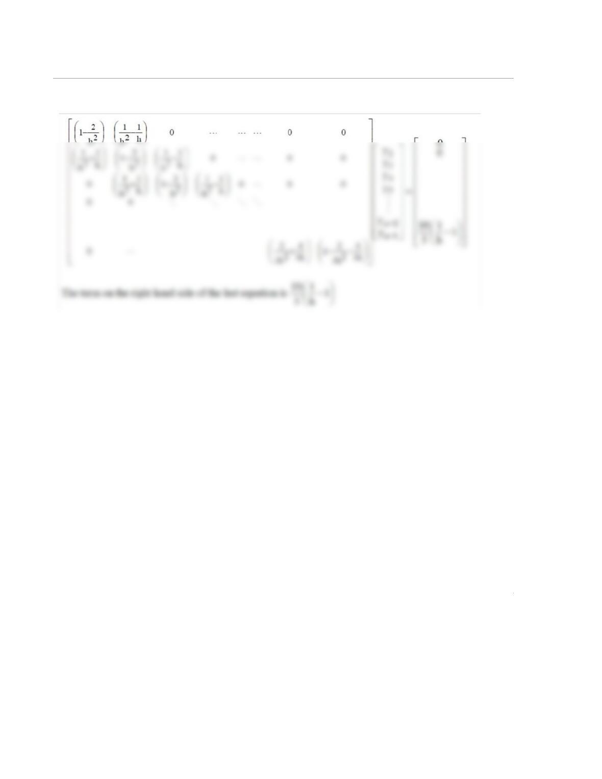
Using Table 8-1, the central difference formula for the derivatives yields:

d2y

dx2

——––2dy

dx

—––

–y+0=

y0() 0=

dy

dx

—––

x1=

5=

x1=

2

1

11.11 Write the BVP in Problem 11.10 as a set of two first-order ODEs, ready to be solved using the

shooting method. Use the linear interpolation method described in Section 11.2 to set up the equation for

determining dy/dx at such that the boundary condition at may be satisfied to a desired error

defined as , where is the calculated value of the derivative at . Set up the

equations to be solved but do not solve.

Solution

x0=

x1=

EH

dyc

dx

——-–

x1=

5–=

dyc

dx

——-–

x1=

1

11.12 Write a user-defined MATLAB function that solves, with the shooting method, a second-order

boundary value problem of the form:

for with and

where and are constants. The function should first calculate two solutions using two assumed values

for the slope at , which are specified by the user, and use these solutions for calculating a new initial

slope using interpolation (Eq. (11.14)), which is then used for calculating the final solution of the problem.

Name the function [x,y]=BVPShootInt(fOFx,gOFx,hOFx,a,b,n,Ya,Yb,WL,WH). The input

arguments fOFx, gOFx, and hOFx are names for the functions that calculate , , and , respec-

tively. They are dummy names for the anonymous or user-defined functions that are imported into BVP-

ShootInt. a and b define the domain of the solution, n is the number of subintervals, Ya and Yb are the

boundary conditions, and WL and WH are the assumed slopes at . Once the first two solutions are cal-

culated, the program should confirm that at the given boundary condition is between the two

solutions, and then calculate the final solution with the interpolated value for the slope. If the boundary

condition at is not between the first two solutions, the program should stop and display an error

message. Use the user-defined function Sys2ODEsRK4 that was written in Example 8-8 for solving the

system of the two first-order ODEs within the user-defined function BVPShootInt.

Use BVPShootInt to solve the boundary value problem in Example 11-6. Use ,

, and .

Solution

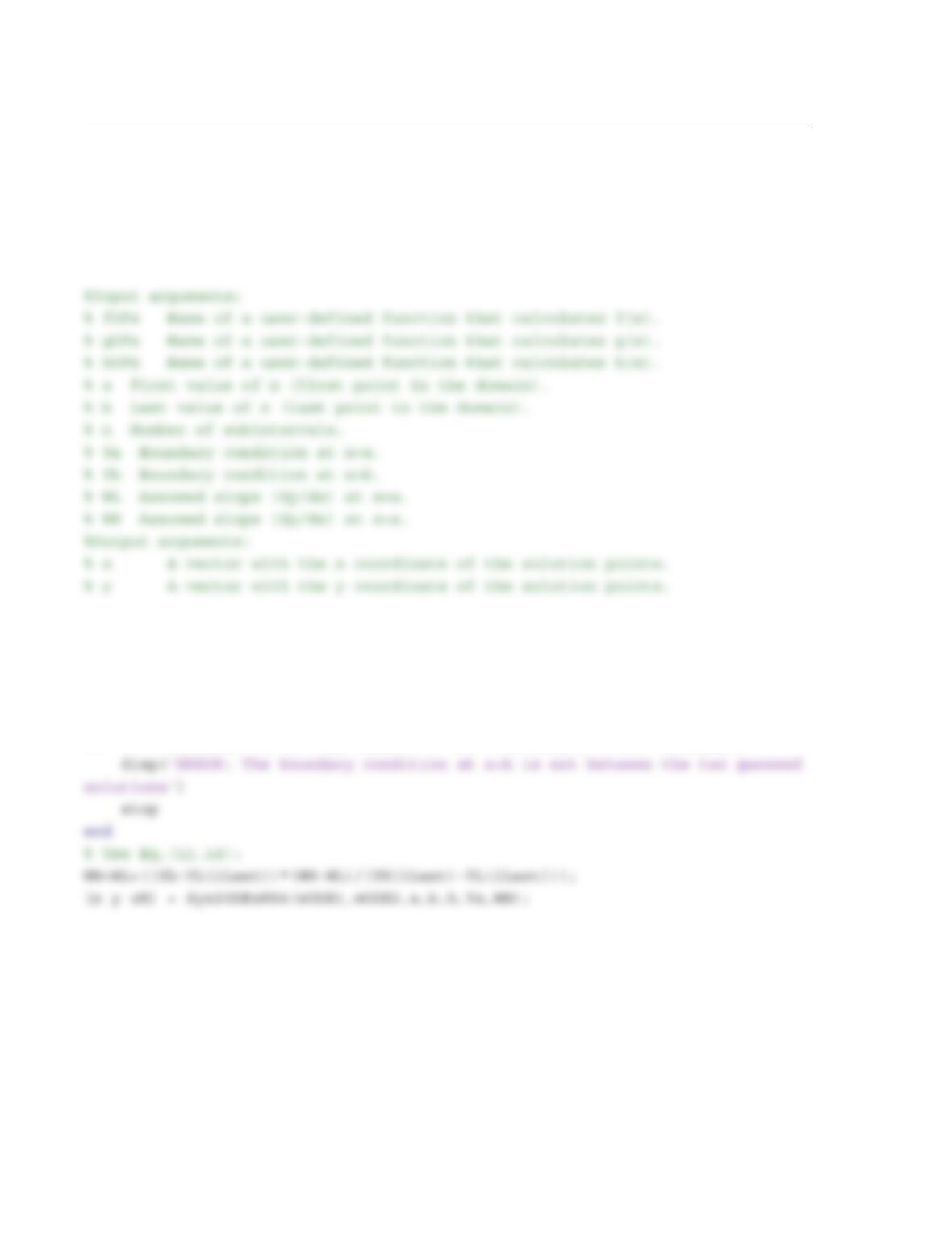
First, the second order ODE is written as a system of two first order ODEs:

d2y

dx2

——-–fx()

dy

dx

—––gx()y++ hx()=

axb≤≤

ya() Ya

=

yb() Yb

=

Ya

Yb

xa=

fx()

gx()

hx()

xa=

xb=

Yb

xb=

n100=

WL5–=

WH1.5–=

dy

dx

—––z=

2

% dy/dx = z

% dz/dx = h(x) – g(x)y – f(x)z

%

%The function uses the user-defined function Sys2ODEsRK4 (Program 10-6)

% to solve the system.

h=(b-a)/n;

[x YL zL] = Sys2ODEsRK4(@ODE1,@ODE2,a,b,h,Ya,WL);

[x YH zH] = Sys2ODEsRK4(@ODE1,@ODE2,a,b,h,Ya,WH);

iLast=length(x);

% Checking if Yb is between the two solutions.

if (Yb < YL(iLast) & Yb < YH(iLast)) | (Yb > YH(iLast) & Yb > YL(iLast))

3

function dydz=ODE1(x,y,z)

dydz=z;

end

function dzdx=ODE2(x,y,z)

dzdx=hOFx(x)-gOFx(x)*y-fOFx(x)*z;

,for (1.1)

with the boundary conditions: and .

In the notation used in the present problem:

, , and .

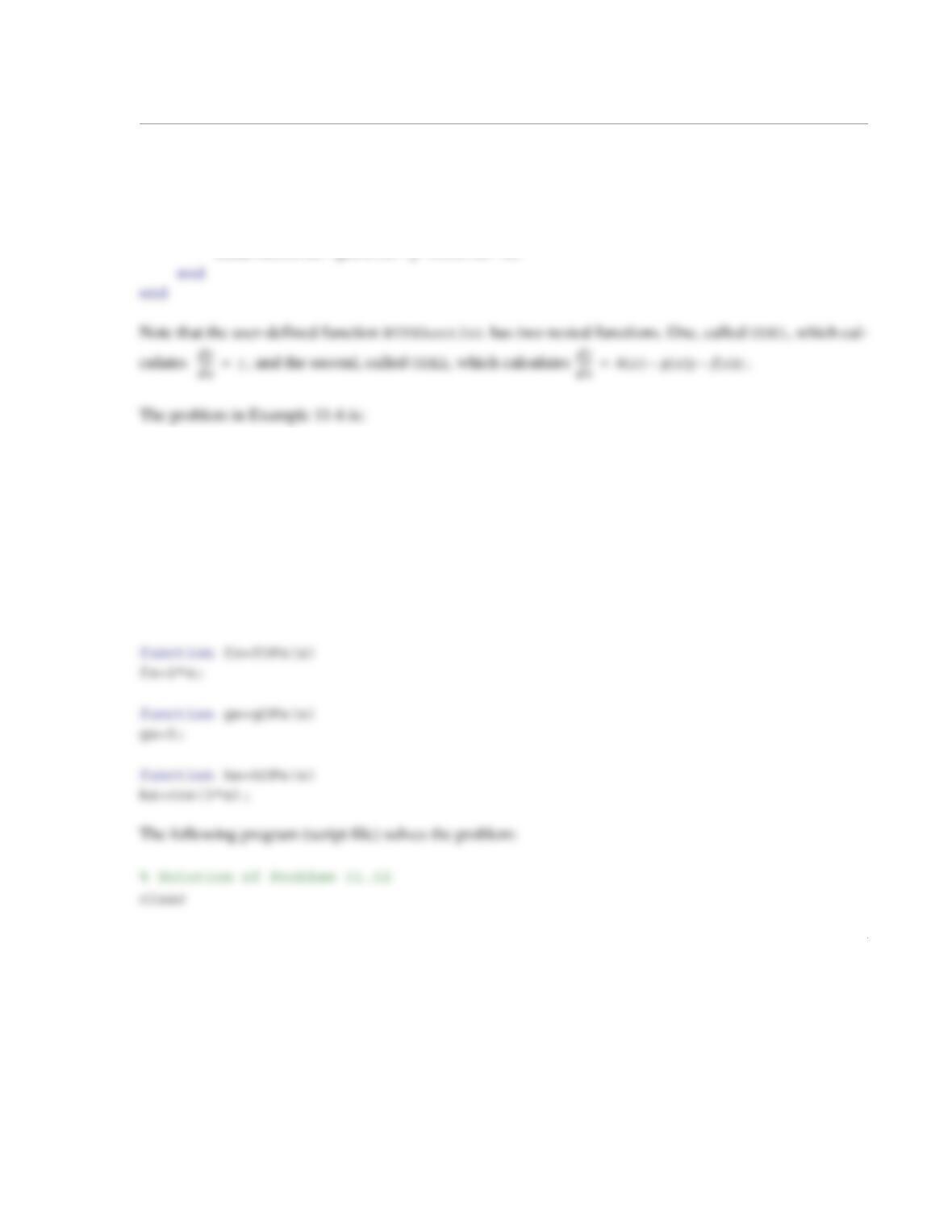
In order to solve the problem, the following three user-defined functions that calculate , and

are created:

d2y

dx2

——-–2xdy

dx

—––5y3x()cos–++ 0=

0xπ≤≤

y0() 1.5=

yπ() 0=

fx() 2x=

gx() 5=

hx() 3x()cos=

fx()

gx()

hx()

4

When the script file is executed, the following figure is displayed in the Figure Window:

0.5

1

1.5

y

1

11.13 Write a user-defined MATLAB function that solves, with the shooting method in conjunction with

the bisection method, a second-order boundary value problem of the form:

for with and

where and are constants. For the function name and arguments use

[x,y]=BVPShootBisec(fOFx,gOFx,hOFx,a,b,n,Ya,Yb,WL,WH). The input arguments

fOFx, gOFx, and hOFx are names for the functions that calculate , , and , respectively. They

are dummy names for the anonymous or user-defined functions that are imported into BVPShootBisec.

a and b define the domain of the solution, n is the number of subintervals, Ya and Yb are the boundary

conditions, and WL and WH are the assumed slopes at that are used in the first two solutions. Once

the first two solutions are calculated, the program should confirm that at the value of the boundary

condition is between the first two solutions. If the boundary condition is not between the first the two

solutions, the program should stop and display an error message. Within the user-defined function BVP-

ShootBisec, use the user-defined function Sys2ODEsRK4 that was written in Example 8-8 for solving

the system of the two first-order ODEs. Iterate until the absolute value of the true error at is smaller

than 0.001.

Use BVPShootBisec to solve the boundary value problem in Example 11-6. Use ,

, and .

Solution

First, the second order ODE is written as a system of two first order ODEs:

d2y

dx2

——-–fx()

dy

dx

—––gx()y++ hx()=

axb≤≤

ya() Ya

=

yb() Yb

=

Ya

Yb

fx()

gx()

hx()

xa=

xb=

Yb

xb=

n100=

WL5–=

WH1.5–=

dy

dx

—––z=

dz

dx

—––hx() gx()y–fx()z–=

2

% dz/dx = h(x) – g(x)y – f(x)z

%

%The function uses the shooting method in conjunction with the bisection

%method, and uses the user-defined function Sys2ODEsRK4 (Program 10-6)

%to solve the system.

h=(b-a)/n;

[x YL zL] = Sys2ODEsRK4(@ODE1,@ODE2,a,b,h,Ya,WL);

[x YH zH] = Sys2ODEsRK4(@ODE1,@ODE2,a,b,h,Ya,WH);

iLast=length(x);

% Checking if Yb is between the two solutions.

if (Yb < YL(iLast) & Yb < YH(iLast)) | (Yb > YH(iLast) & Yb > YL(iLast))

disp(‘ERROR: The boundary condition at x=b is not between the two guessed

solutions’)

3

end

if i > imax

fprintf(‘Solution was not obtained in %i iterations.\n’,imax)

end

function dydx=ODE1(x,y,z)

dydx=z;

end

function dzdx=ODE2(x,y,z)

dzdx=hOFx(x)-gOFx(x)*y-fOFx(x)*z;

4

are created:

function fx=fOFx(x)

fx=2*x;

The following program (script file) solves the problem:

clear all

a=0; b=pi; n=100; Ya=1.5; Yb=0;

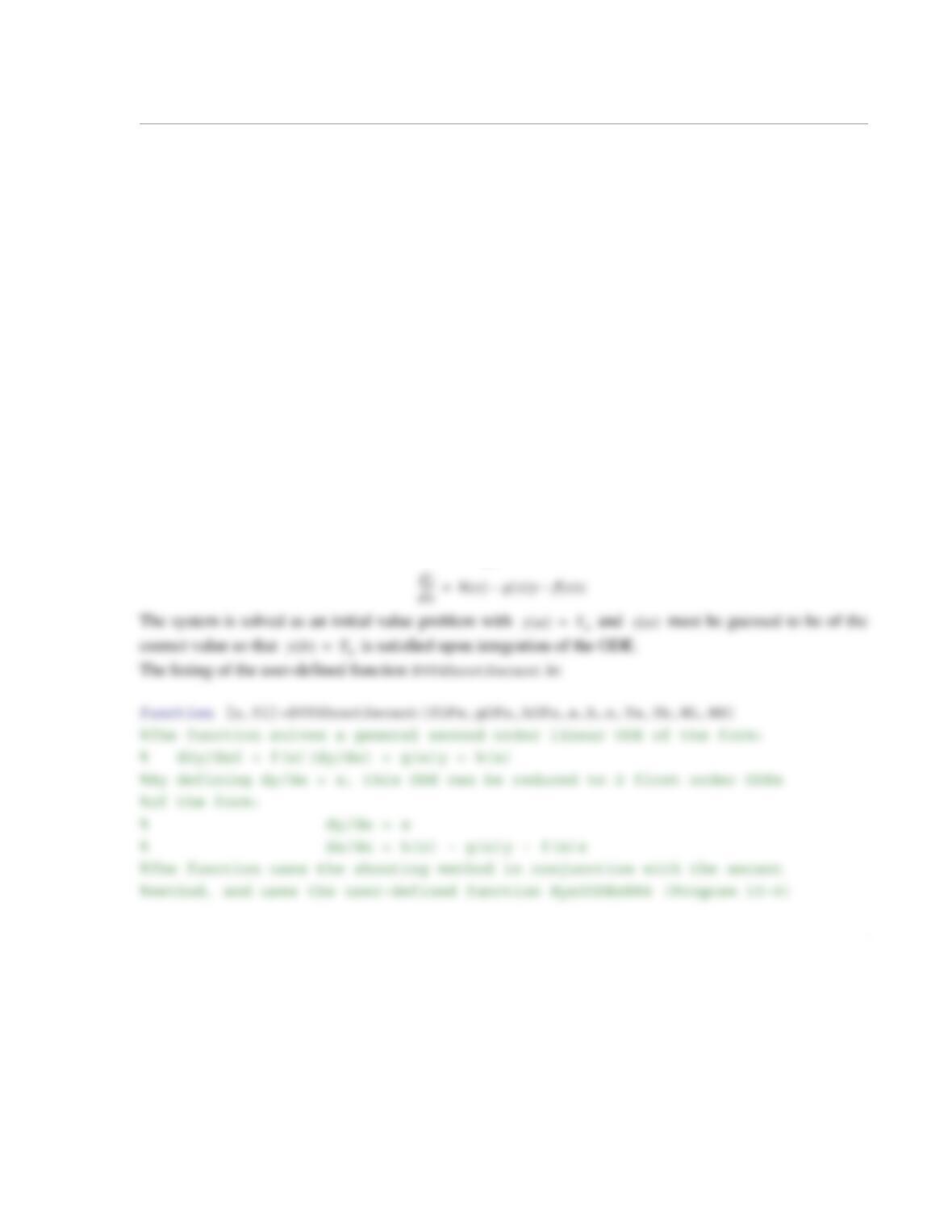
When the script file is executed, the following figure is displayed in the Figure Window:

1

1.5

1

11.14 Write a user-defined MATLAB function that solves, with the shooting method in conjunction with

the secant method, a second-order boundary value problem of the form:

for with and

where and are constants. For the function name and arguments use

[x,y]=BVPShootSecant(fOFx,gOFx,hOFx,a,b,n,Ya,Yb,WL,WH). The input arguments

fOFx, gOFx, and hOFx are names for the functions that calculate , , and , respectively. They

are dummy names for the anonymous or user-defined functions that are imported into

BVPShootSecant. The arguments a and b define the domain of the solution, n is the number of subin-

tervals, Ya and Yb are the boundary conditions, and WL and WH are the assumed slopes at that are

used in the first two solutions. Within the user-defined function BVPShootSecant, use the user-defined

function Sys2ODEsRK4 that was written in Example 10-8 for solving the system of the two first-order

ODEs. Iterate until the absolute value of the true error at is smaller than 0.001.

Use BVPShootSecant to solve the boundary value problem in Example 11-6. Use ,

, and .

Solution

First, the second order ODE is written as a system of two first order ODEs:

d2y

dx2

——-–fx()

dy

dx

—––gx()y++ hx()=

axb≤≤

ya() Ya

=

yb() Yb

=

Ya

Yb

fx()

gx()

hx()

xa=

xb=

n100=

WL5–=

WH1.5–=

dy

dx

—––z=

2

%to solve the system.

%Input arguments:

% fOFx Name of a user-defined function that calculates f(x).

% gOFx Name of a user-defined function that calculates g(x).

% hOFx Name of a user-defined function that calculates h(x).

h=(b-a)/n;

[x YL zL] = Sys2ODEsRK4(@ODE1,@ODE2,a,b,h,Ya,WL);

[x YH zH] = Sys2ODEsRK4(@ODE1,@ODE2,a,b,h,Ya,WH);

iLast=length(x);

% Start iterations using the secant method

imax=15; tol=0.001;

W(1)=WL; W(2)=WH; E(1)=YL(iLast) – Yb; E(2)=YH(iLast) – Yb;

for i = 2:imax + 1

3

end

Note that the user-defined function BVPShootSecant has two nested functions. One, called ODE1, which

calculates , and the second, called ODE2, which calculates .

The problem in Example 11-6 is:

,for (1.1)

dy

dx

—––z=

dz

dx

—––hx() gx()y–fx()z–=

d2y

dx2

——-–2xdy

dx

—––5y3x()cos–++ 0=

0xπ≤≤