Chapter 4 Homework Carry out the first three iterations of the solution

1

4.15 Carry out the first three iterations of the solution of the following system of equations using the

Gauss–Seidel iterative method. For the first guess of the solution, take the value of all the unknowns to be

zero.

Solution

The essence of the Gauss-Seidel iterative method is given by Eq. (4.51):

8x12x23x3

++ 51=

2x15x2x3

++ 23=

3x1

–x26x3

++ 20=

xi

1

aii

—– biaij xj

j1=

ji≠

jn=









–=

i12…n,, ,=

1

4.16 Carry out the first three iterations of the solution of the following system of equations using the

Gauss–Seidel iterative method. For the first guess of the solution, take the value of all the unknowns to be

zero.

Solution

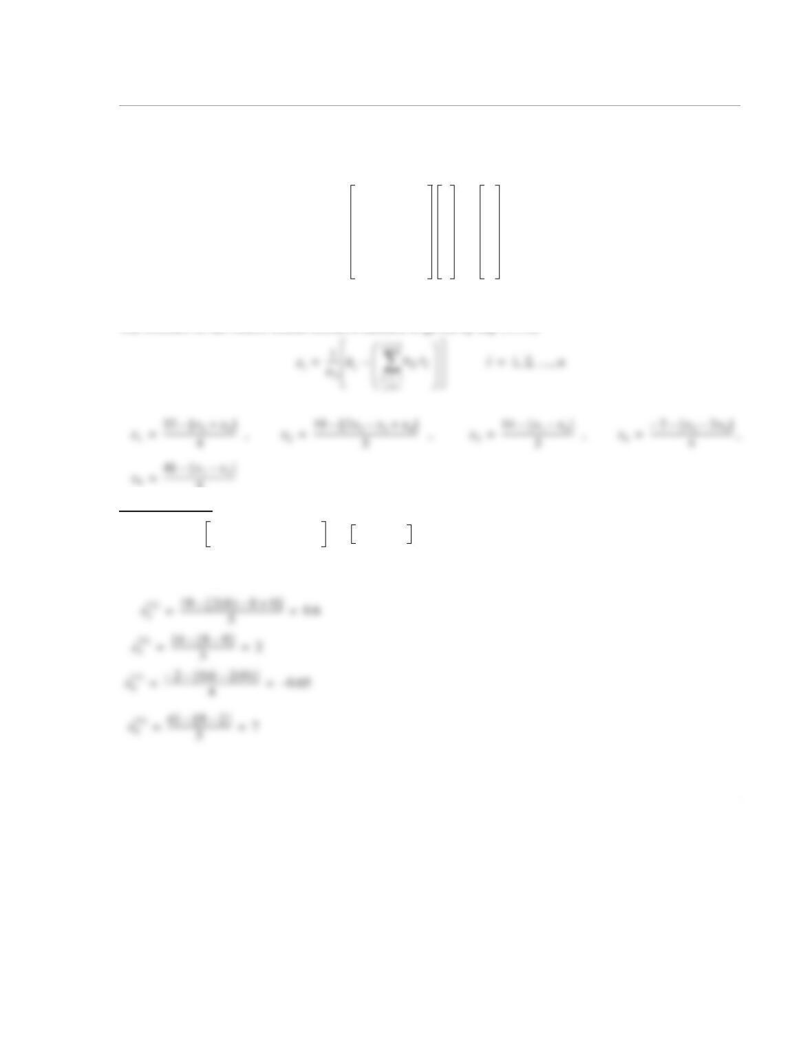
The essence of the Gauss-Seidel iterative method is given by Eq. (4.51):

First Iteration:

Starting with ,

40 1 0 1

25 1–10

10 3 1–0

01 0 4 2–

10 1–05

x1

x2

x3

x4

x5

32

19

14

2–

41

=

5

x1

0()x2

0()x3

0()x4

0()x5

0() 00000

=

x1

1() 32 0 0+[]–

4

—————–———––8==

2

Second Iteration:

Starting with ,

Third Iteration:

Starting with ,

x1

0()x2

0()x3

0()x4

0()x5

0() 80.62 0.65–7

=

x1

2() 32 2 7+[]–

4

—————-————–5.75==

x1

0()x2

0()x3

0()x4

0()x5

0() 5.75 2.03 2.5333 2.4925 7.5567

=

x1

3() 32 2.5333 7.5567+[]–

4

—————–———————————–—–5.4775==

1

4.17 Find the condition number of the matrix in Problem 4.13 using the infinity norm.

Solution

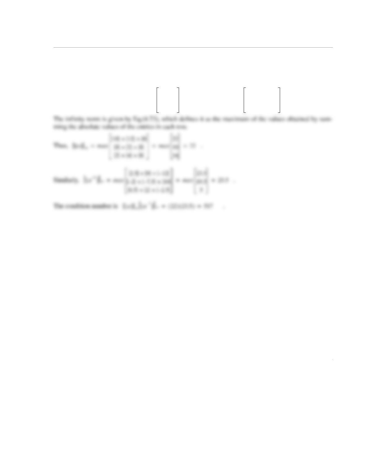
The matrix in Problem 4.13 is . Its inverse is .

a[]

10 12 0

028

248

=

a1–

[]

2.5 9 12–

2–7.5–10

0.5 2 2.5–

=

1

4.18 Find the condition number of the matrix in Problem 4.14 using the infinity norm.

Solution

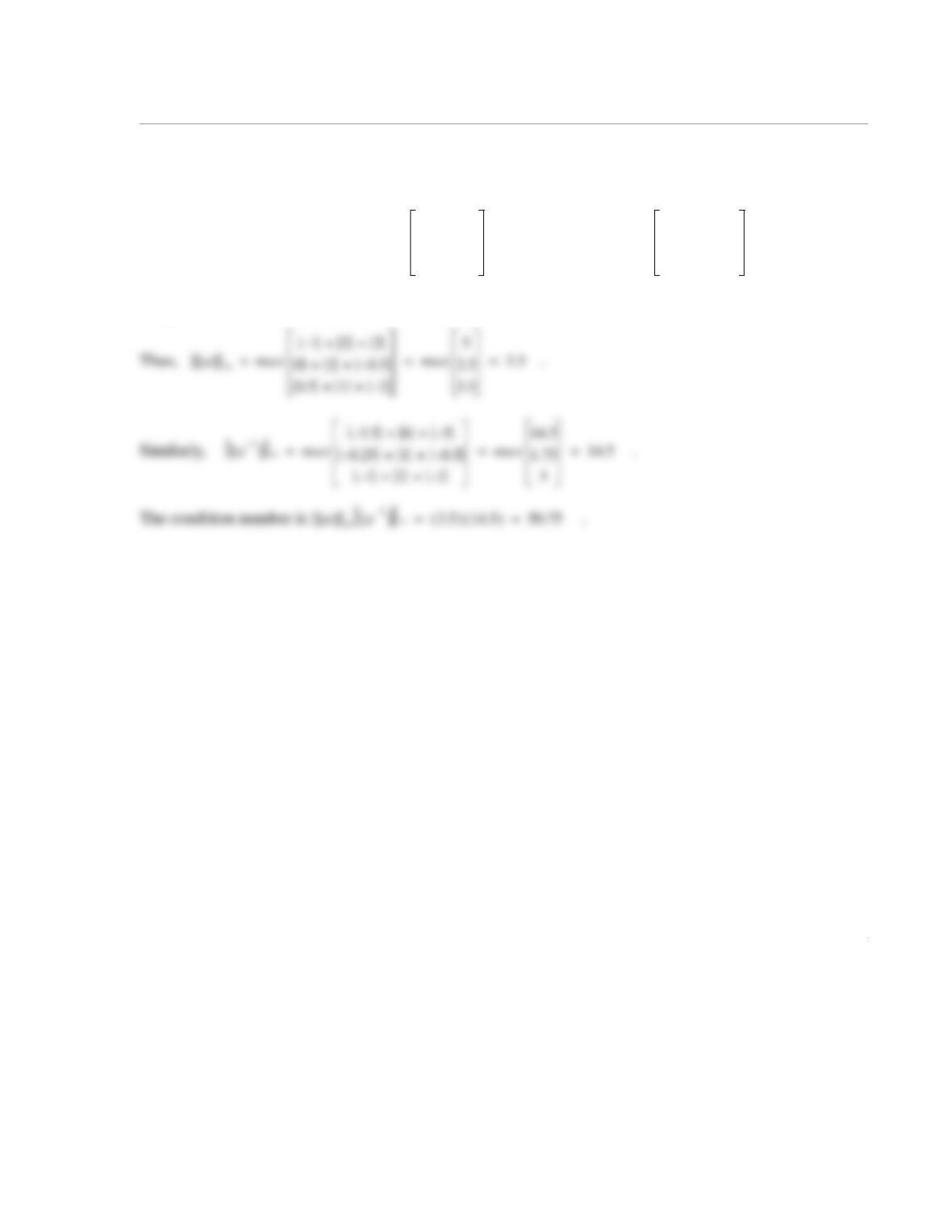
The matrix in Problem 4.14 is . Its inverse is .

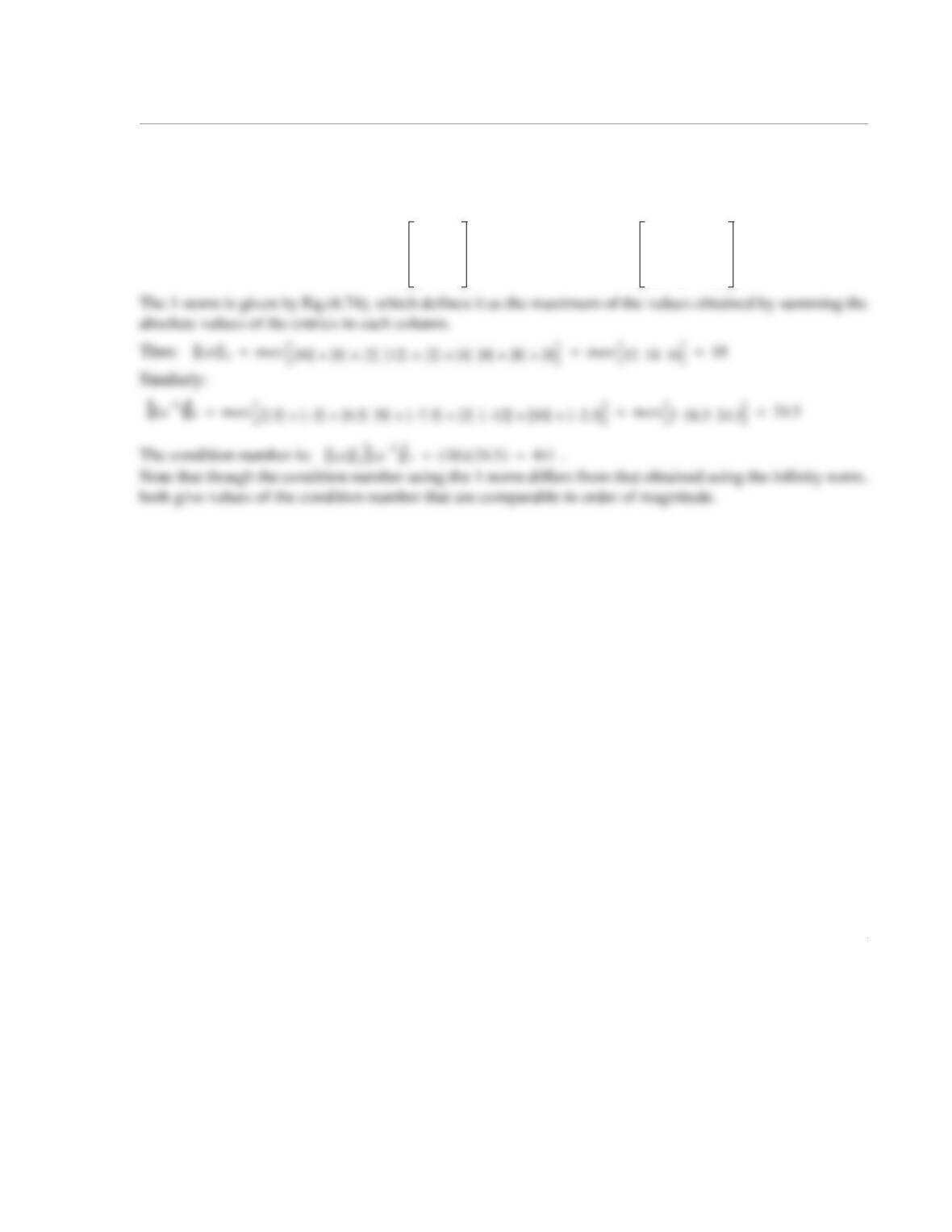
The infinity norm is given by Eq.(4.73), which defines it as the maximum of the values obtained by sum-

ming the absolute values of the entries in each row.

a[]

1–22

02 0.5–

0.5 1 2–

=

a1–

[]

3.5–65–

0.25– 1 0.5–

1–22–

=

1

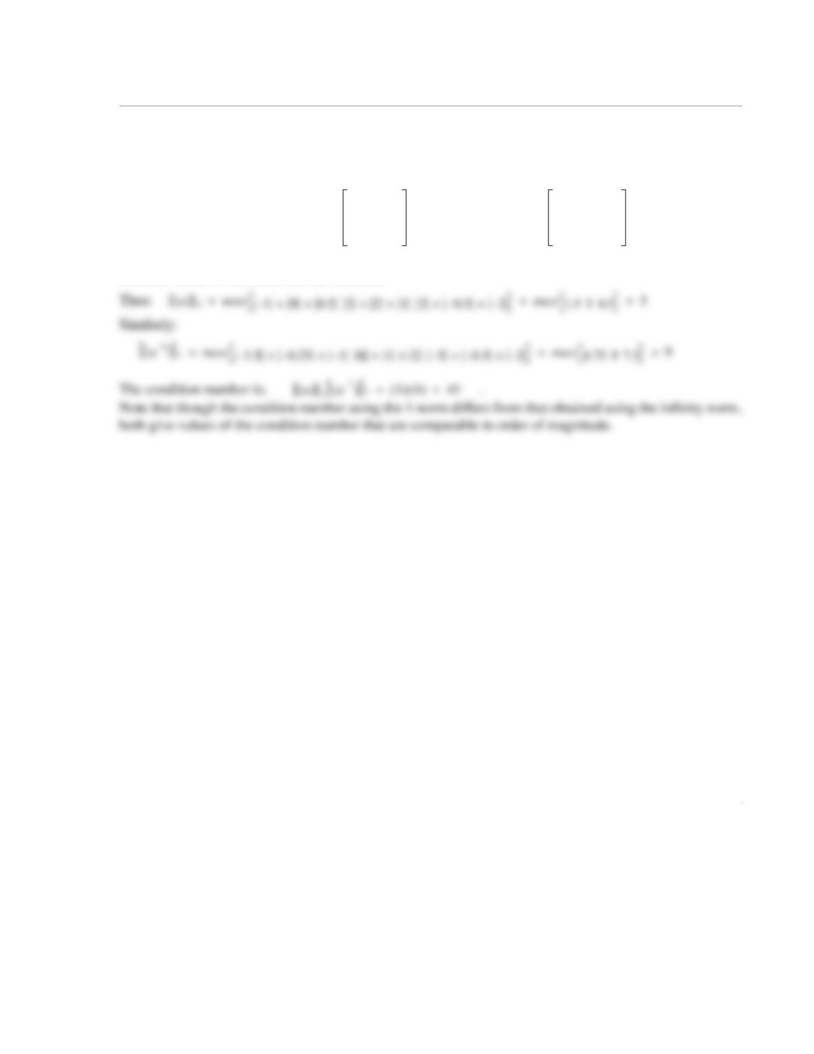
4.19 Find the condition number of the matrix in Problem 4.13 using the 1-norm.

Solution

The matrix in Problem 4.13 is . Its inverse is .

a[]

10 12 0

028

248

=

a1–

[]

2.5 9 12–

2–7.5–10

0.5 2 2.5–

=

1

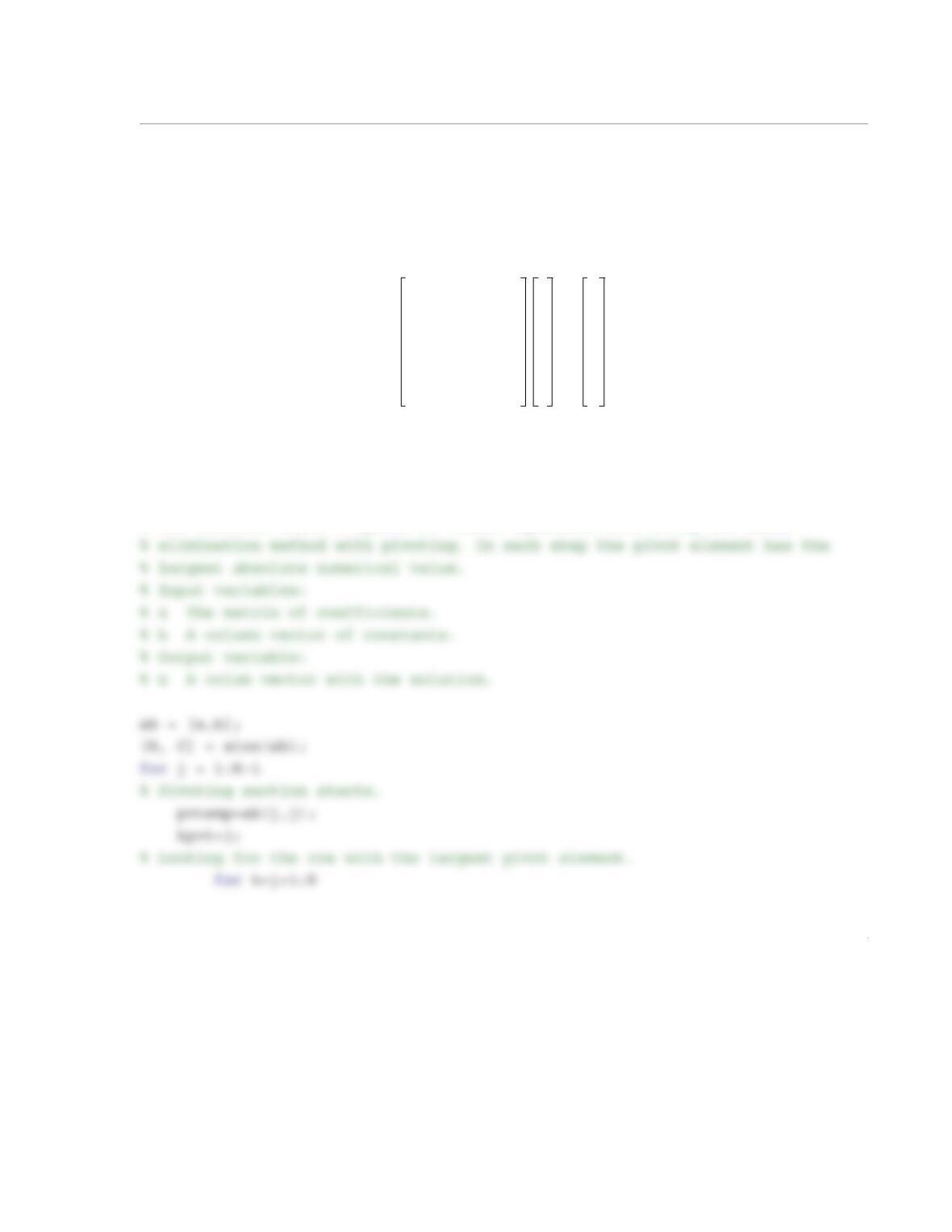
4.20 Find the condition number of the matrix in Problem 4.14 using the 1-norm.

Solution

The matrix in Problem 4.14 is . Its inverse is .

The 1-norm is given by Eq.(4.74), which defines it as the maximum of the values obtained by summing the

absolute values of the entries in each column.

a[]

1–22

0 2 0.5–

0.5 1 2–

=

a1–

[]

3.5–65–

0.25– 1 0.5–

1–22–

=

1

4.21 Modify the user-defined function GaussPivot in Program 4-2 (Example 4-3) such that in each

step of the elimination the pivot row is switched with the row that has a pivot element with the largest

absolute numerical value. For the function name and arguments use x = GaussPivotLarge(a,b),

where a is the matrix of coefficients, b is the right-hand-side column of constants, and x is the solution.

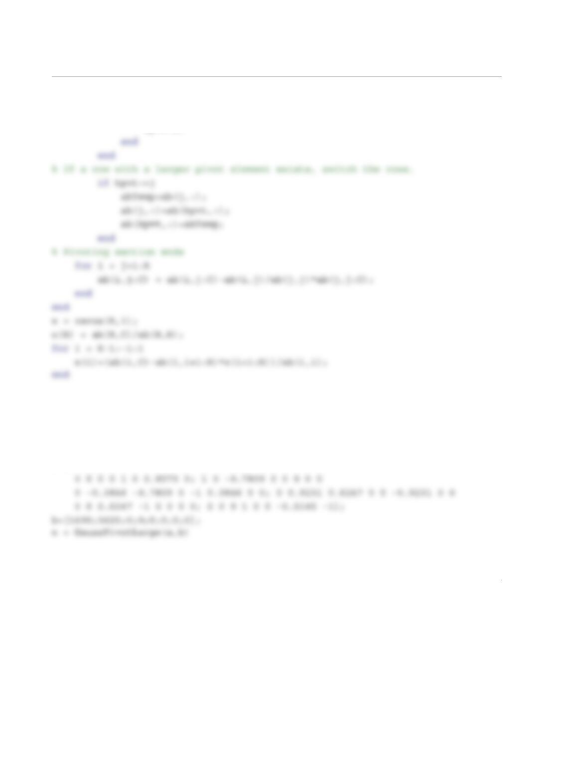
(a) Use the GaussPivotLarge function to solve the system of linear equations in Eq. (4.17).

(b) Use the GaussPivotLarge function to solve the system:

Solution

The listing of the user-defined function GaussPivotLarge is:

function x = GaussPivotLarge(a,b)

% The function solve a system of linear equations ax=b using the Gauss

03 8 5–1–6

312 4–852–

80 010 3–7

310004

00 4 6–02

30500 6–

x1

x2

x3

x4

x5

x6

34

20

45

36

60

28

=

2

if ab(k,j)~=0 & abs(ab(k,j)) > abs(pvtemp)

pvtemp=ab(k,j);

kpvt=k;

(a) The following program (script file) uses the user-defined GaussPivotLarge function to solve the

system of linear equations in Eq. (4.17).

% Solution of HW4_21a, script

clear all

a=[0 0.9231 0 0 0 0 0 0; -1 -0.3846 0 0 0 0 0 0

3

When the program is executed, the following result is displayed in the Command Window.

>> format short e

x =

-4.3291e+003

(b) The following program (script file) uses the user-defined GaussPivotLarge function to solve the

system of linear equations that is given in the problem statement.

% Solution of HW4_21b, script

clear all

a =[0 3 8 -5 -1 6; 3 12 -4 8 5 -2; 8 0 0 10 -3 7

3 1 0 0 0 4; 0 0 4 -6 0 2; 3 0 5 0 0 -6];

b = [34; 20; 45; 36; 60; 28];

x = GaussPivotLarge(a,b)

When the program is executed, the following result is displayed in the Command Window.

1

4.22 Write a user-defined MATLAB function that solves a system of n linear equations, ,

with the Gauss–Jordan method. The program should include pivoting in which the pivot row is switched

with the row that has a pivot element with the largest absolute numerical value. For the function name and

arguments use x = GaussJordan(a,b), where a is the matrix of coefficients, b is the right-hand-side

column of constants, and x is the solution.

(a) Use the GaussJordan function to solve the system:

(b) Use the GaussJordan function to solve the system:

Solution

The listing of the user-defined function GaussJordan is:

a[]x[] b[]=

2x1x24x32x4

–++ 19=

3x–14x22x3x4

–++ 1=

3x15x22x3

–x4

++8=

2x–13x22x34x4

+++ 13=

12 3456

13–254–6

61 2–435

32 1–456

42–1–365

56–3–42–1

x1

x2

x3

x4

x5

x6

91

37

63

81

69

4–

=

2

% Pivoting section starts

pvtemp=ab(j,j);

kpvt=j;

% If a row with a larger pivot element exists, switch the rows.

if kpvt~=j

abTemp=ab(j,:);

ab(j,:)=ab(kpvt,:);

ab(kpvt,:)=abTemp;

end

% Pivoting section ends

ab(j,:)= ab(j,:)/ab(j,j);

for i = 1:R

if i~=j

ab(i,j:C) = ab(i,j:C)-ab(i,j)*ab(j,j:C);

end

3

When the program is executed, the following result is displayed in the Command Window.

x =

3

1

4

2

(b) The following program (script file) uses the user-defined GaussJordan function to solve the system

of linear equations that is given in the problem statement.

1

4.23 Write a user-defined MATLAB function that decomposes an matrix into a lower triangular

matrix and an upper triangular matrix (such that ) using the Gauss elimination

method (without pivoting). For the function name and arguments, use [L,U] = LUdecompGauss(A),

where the input argument A is the matrix to be decomposed and the output arguments L and U are the cor-

responding upper and lower triangular matrices. Use LUdecompGauss to determine the LU decomposi-

tion of the following matrix:

Solution

The listing of the user-defined function GaussJordan is:

function [L,U] = LUdecompGauss(A)

% The function decomposes a matrix into lower and upper triangular

nn×

A[]

L[]

U[]

A[] L[]U[]=

41–32

8–03–3.5–

23.5–103.75

8–4– 1 0.5–

2

U=A;

The following program (script file) uses the user-defined LUdecompGauss to decompose the matrix given

in the problem.

clear,clc

A=[4 -1 3 2; -8 0 -3 -3.5; 2 -3.5 10 3.75; -8 -4 1 -0.5]

[L,U] = LUdecompGauss(A)

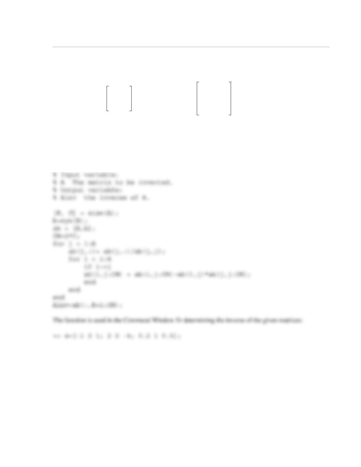
The following result is displayed in the Command Window when the script is executed:

A =

1

4.24 Write a user-defined MATLAB function that determines the inverse of a matrix using the Gauss–Jor–

dan method. For the function name and arguments use Ainv = Inverse(A), where A is the matrix to be

inverted, and Ainv is the inverse of the matrix. Use the Inverse function to calculate the inverse of:

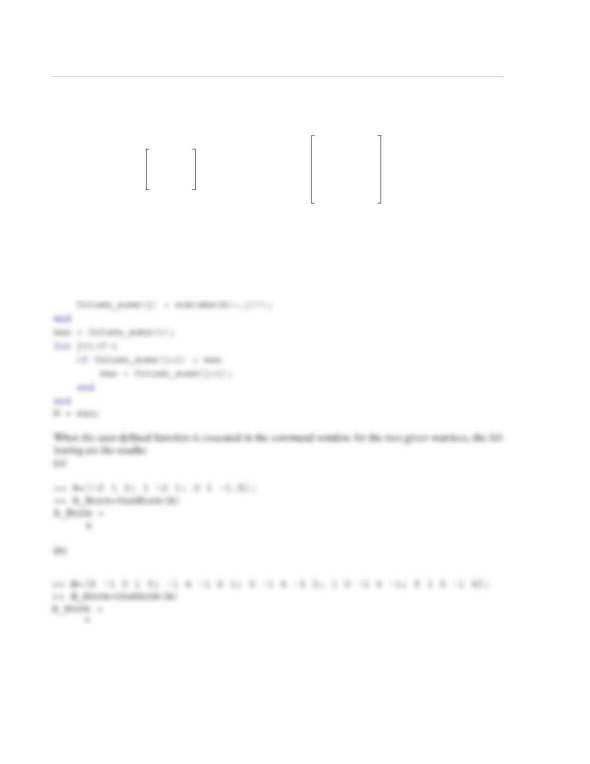
(a) The matrix . (b) The matrix .

Solution

The listing of the user-defined function Inverse is:

function Ainv = Inverse(A)

% The function solve a system of linear equations ax=b using the Gauss

% elimination method.

1–21

22 4–

0.210.5

1–2–12

11 4–2–

12–4–2–

24–12–

2

>> ainv = Inverse(a)

ainv =

-0.7143 0 1.4286

0.2571 0.1000 0.2857

-0.2286 -0.2000 0.8571

2

7

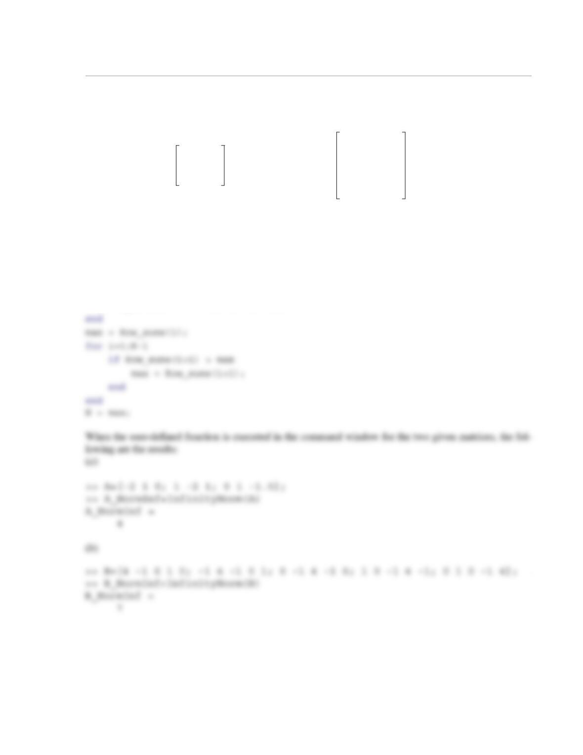
4.25 Write a user-defined MATLAB function that calculates the 1-norm of any matrix. For the function

name and arguments use N = OneNorm(A), where A is the matrix and N is the value of the norm. Use the

function for calculating the 1-norm of:

(a) The matrix . (b) The matrix .

Solution

The user-defined function is:

function N = OneNorm(A)

[R,C]=size(A);

for j=1:C

A

2–1 0

12–1

0 1 1.5–

=

B

41–010

1–41–01

01–41–0

10 1–41–

010 1–4

=

1

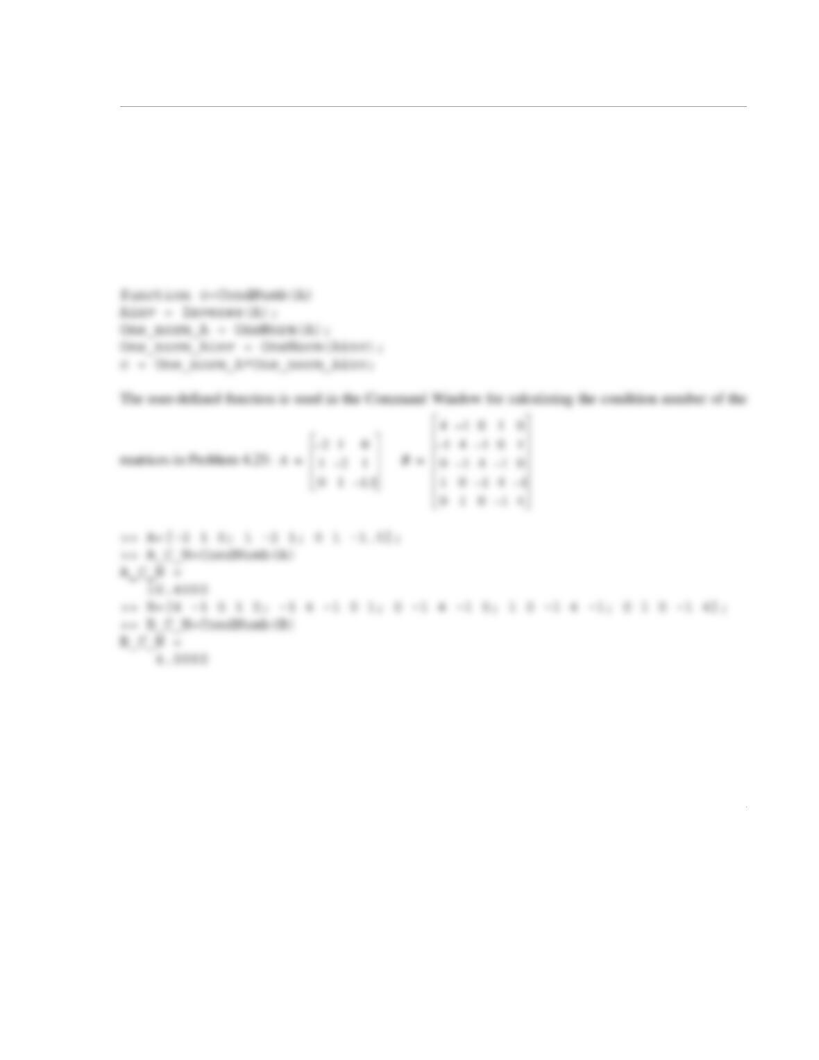
4.26 Write a user-defined MATLAB function that calculates the infinity norm of any matrix. For the func-

tion name and arguments use N = InfinityNorm(A), where A is the matrix, and N is the value of the

norm. Use the function for calculating the infinity norm of:

(a) The matrix . (b) The matrix .

Solution

The user-defined function is:

function N = InfinityNorm(A)

[R,C]=size(A);

for i=1:R

Row_sums(i) = sum(abs(A(i,:)));

A

2–10

12–1

0 1 1.5–

=

B

41–010

1–41–01

01–41–0

10 1–41–

010 1–4

=

1

4.27 Write a user-defined MATLAB function that calculates the condition number of an matrix by

using the 1-norm. For the function name and arguments use c = CondNumb_One(A), where A is the

matrix and c is the value of the condition number. Within the function, use the user-defined functions

Inverse from Problem 4.24 and OneNorm from Problem 4.25. Use the function CondNumb_One for

calculating the condition number of the matrices in Problem 4.25.

Solution

The listing of the user-defined function CondNumb is:

nn×()