1
5.1 Show that the eigenvalues of the identity matrix are the number 1 repeated n times.
Solution
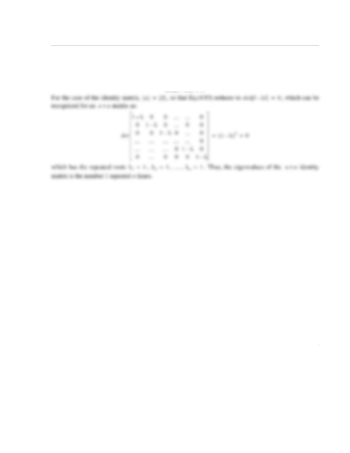
The eigenvalues of any matrix are determined from the solution of the characteristic equation, Eq.(4.93):
nn×
det a λI–[]0=
1
5.2 Show that the eigenvalues of the following matrix are .
Solution
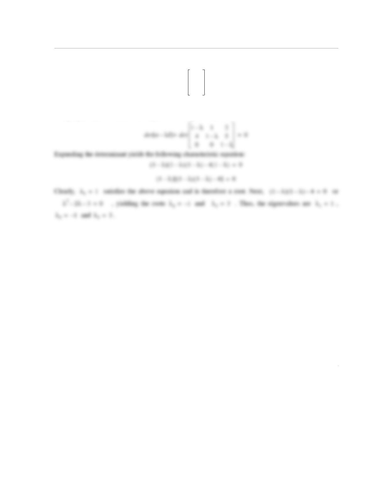
Using Eq.(5.93), the characteristic equation for the given matrix is:
31–1,,
112
415
001
1
5.3 Find the eigenvalues of the following matrix by solving for the roots of the characteristic equation.
Solution
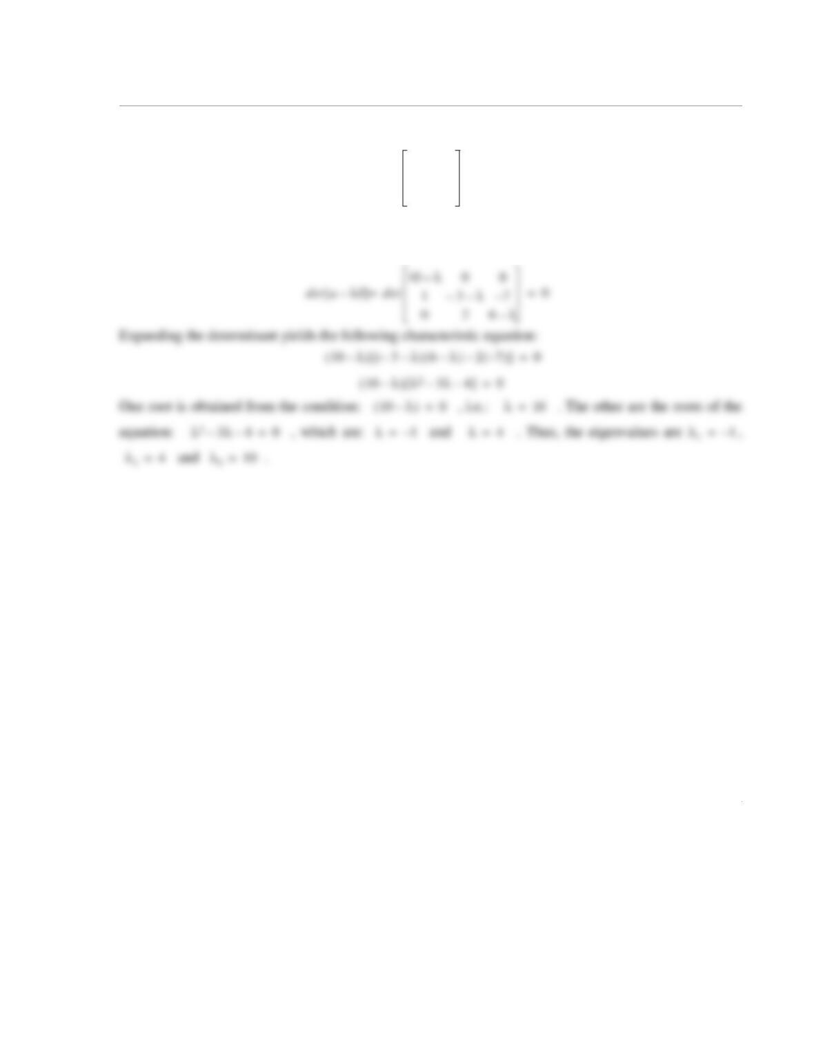
Using Eq.(5.93), the characteristic equation for the given matrix is:
10 0 0
13–7–
026
1
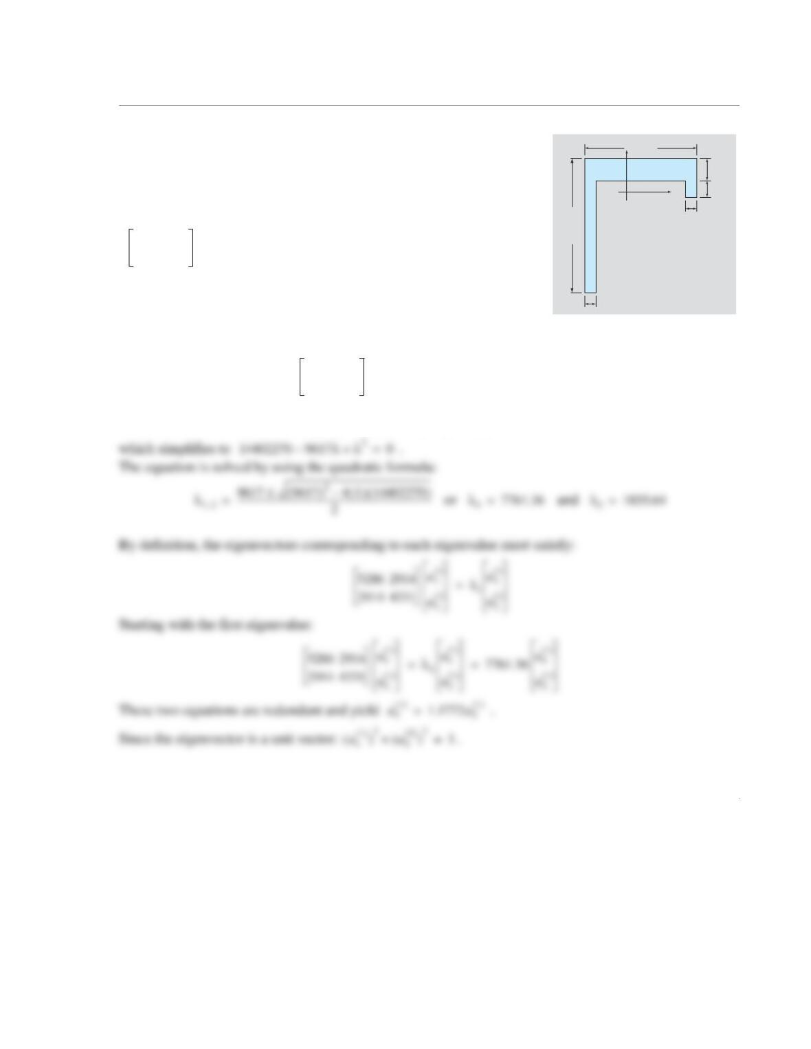
5.4 The moment of inertia , , and the product of inertia of the
cross-sectional area shown in the figure are:
mm4, mm
4,and mm
4
The principal moments of inertia are the eigenvalues of the matrix
, and the principal axes are in the direction of the eigen-
vectors. Determine the principal moments of inertia by solving the char-
acteristic equation. Determine the orientation of the principal axes of
inertia (unit vectors in the directions of the eigenvectors).
Solution
The eigenvalues of the matrix are the principal moments of inertia. They are determined from
the roots of the characteristic equation:
4 mm
O
y
x
24 mm
2 mm
20 mm
3 mm
2 mm
Ix
Iy
Ixy
Ix5286=
Iy4331=
Ixy 2914=
5286 2914
2914 4331
5286 2914
2914 4331
5286 λ–()4331 λ–()2914()2914()–0=
2
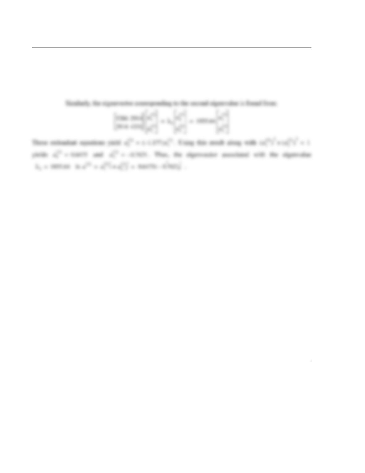
Combining the two equations yields: and
Thus, the eigenvector associated with the eigenvalue is
.
u2
1() 0.6474=
u1
1() 0.7621=
λ17761.36=
u1() u1
1()
i
ˆu2
1()
j
ˆ
+ 0.7621i
ˆ0.6474 j
ˆ
+==
u1
1
5.5 Determine the principal moments of inertia of the cross-sectional area in Problem 5.4 by using the
QR factorization and iteration method. Carry out the first four iterations.
Solution
This is done in the MATLAB command window to preserve precision:
>> c=[5286;2914]; e=[1;0];
>> norm_c=sqrt((c(1)^2)+(c(2)^2)); v=c+(norm_c*e);
>> vT_v=v’*v; v_vT=v*v’; I=eye(2); H=I-((2/vT_v)*v_vT);
>> A=[5286 2914;2914 4331]; Q1=H; R1=H*A;
>> Q1*R1
ans =
2
A4 =
1.0e+003 *
7.7606 -0.0686
-0.0686 1.8564
>> c=[7760.6;-68.6]; e=[1;0]; norm_c=sqrt((c(1)^2)+(c(2)^2));
>> v=c+(norm_c*e);
1
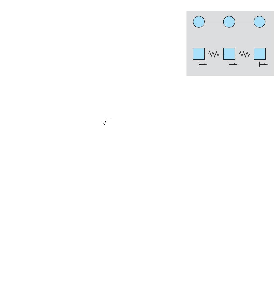
5.6 The structure of an BeCl2 molecule may be idealized as three
masses connected by two springs, where the masses are the beryllium
and chlorine atoms, and the springs represent the chemical bond
between the beryllium and chlorine atoms.The equation of motion for
each atom (mass) may be written as:
where k is the restoring force spring constant representing the Be–Cl bonds. Since the molecule is free to
vibrate, normal mode (i.e., along the axis) vibrations can be examined by substituting , where
is the amplitude of the jth mass, , is the frequency, and t is time. This results in the following
system of equations:
(5.57)
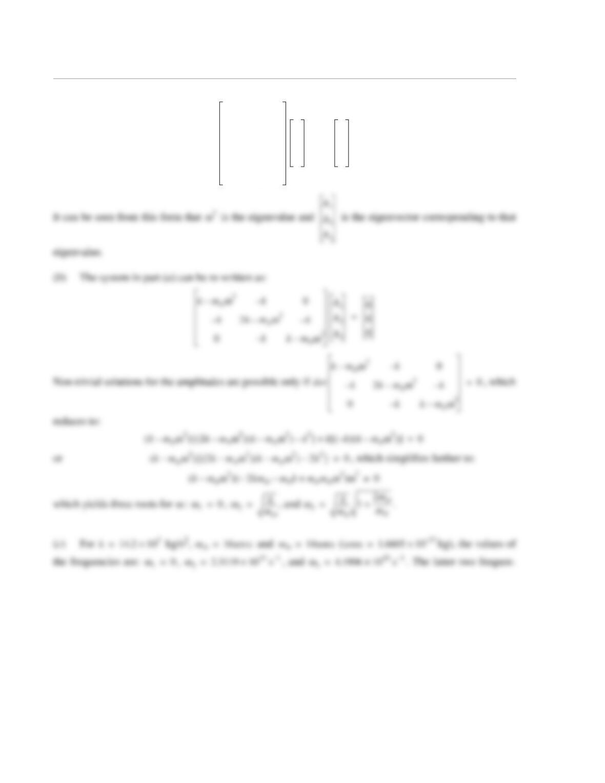
(a) Rewrite the system of equations in Eq. (5.57) as an eigenvalue problem, and show that the quantity
is the eigenvalue.
(b) Write the characteristic equation and solve for the different frequencies when kg/
s2, kg, and kg.
(c) Find the wavelengths (where m/s is the speed of light in vacuum) that corre-
spond to the frequencies from part (b). Express the answers in units of microns or m (where
m).
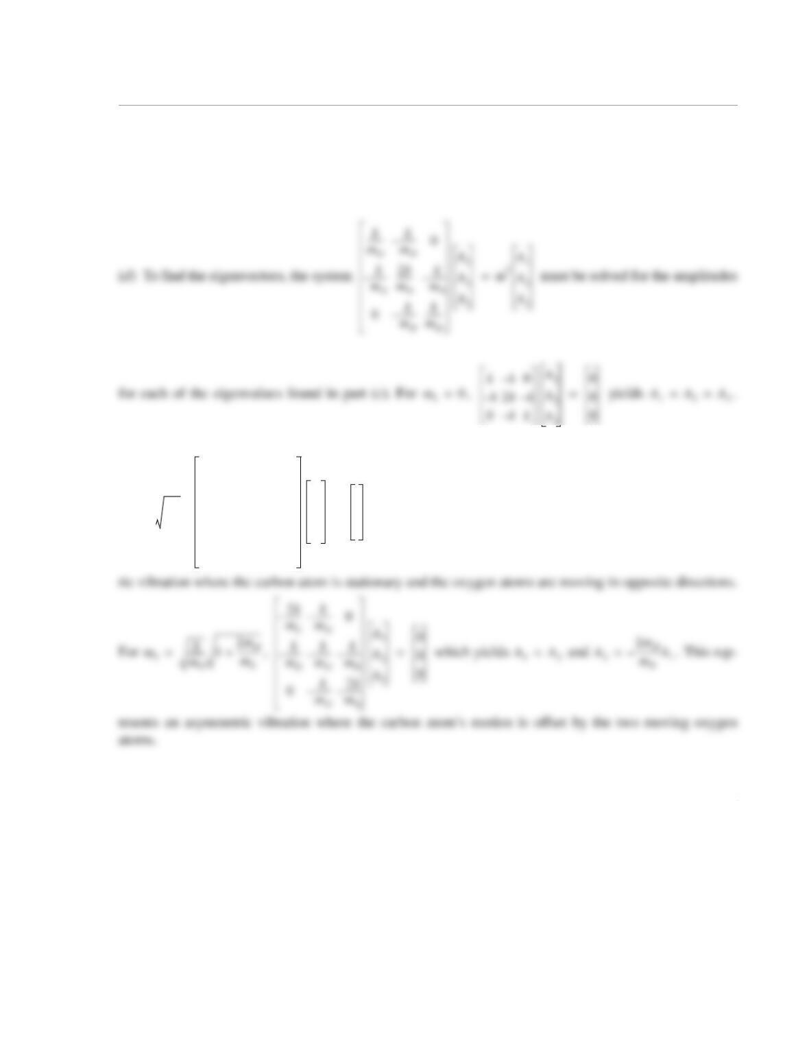
(d) Determine the eigenvectors corresponding to the eigenvalues found in part (c). From the eigenvectors,
deduce the relative motion of the atoms (i.e., are they moving toward or away from each other?)
Solution
(a) The system of equations (5.57) can be re-written in the following matrix form:
Be Cl
Cl
x2x3
x1
mCl mCl
mBe
mCl
d2x1
dt2
———– kx1
–kx2
+=
mBe
d2x2
dt2
———– 2kx2
–kx1kx3
++=
mCl
d2x3
dt2
———– kx2kx3
–=
xjAjeiωt
=
Aj
i1–=
ω
ω2A1
–k
mCl
——-– A1
–k
mCl
——-– A2
+=
ω2A2
–2k
mBe
——––A2
–k
mBe
——––A1
k
mBe
——––A3
++=
ω2A3
–k
mCl
——-– A2
k
mCl
——-– A3
–=
ω2
ω
k1.81 102
×=
mCl 35.45 1.6605 10 27–
××=
mBe 9.01 1.6605×10 27–
×=
λ2πc
ω
——––
=
c310
8
×=
µ
1µm10
6–
=
2
k
mO
——– k
mO
——–
–0
k
mN
——–
–2k
mN
——–k
mN
——–
–
0k
mO
——–
–k
mO
——–
A1
A2
A3
ω2
A1
A2
A3
=
3
cies correspond to wavelengths of or and or
. It turns out that one of the wavelengths ( µm) is observed in the absorption spectrum
of the NO2 molecule.
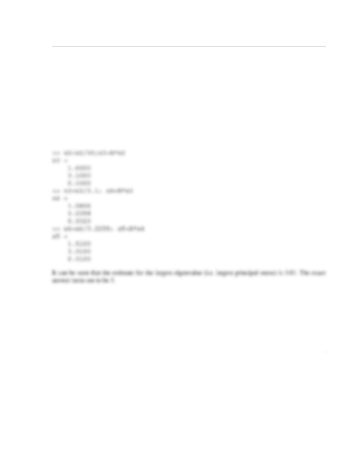
This represents translation of the entire molecule, with no relative motion between the atoms. For
, which yields and . This represents a symmet-
ω3
A1A3
λ28.2 10 6–
× m=
λ28.2 µm=
λ34.5 10 6–
× m=
λ34.5 µm=
λ4.3=
ω2
k
mO
——–=
0k
mO
——–
–0
k
mN
——–
–2k
mN
——–k
mO
——–
–k
mN
——–
–
k
mO
——–
–k
mO
——–
–k
mO
——–
A1
A2
A3
0
0
0
=
A20=
A1A3
–=
A1A2A3
1
5.7 Apply the power method to find the largest eigenvalue of the matrix from Problem 5.2 starting with the
vector [1 1 1]T.
Solution
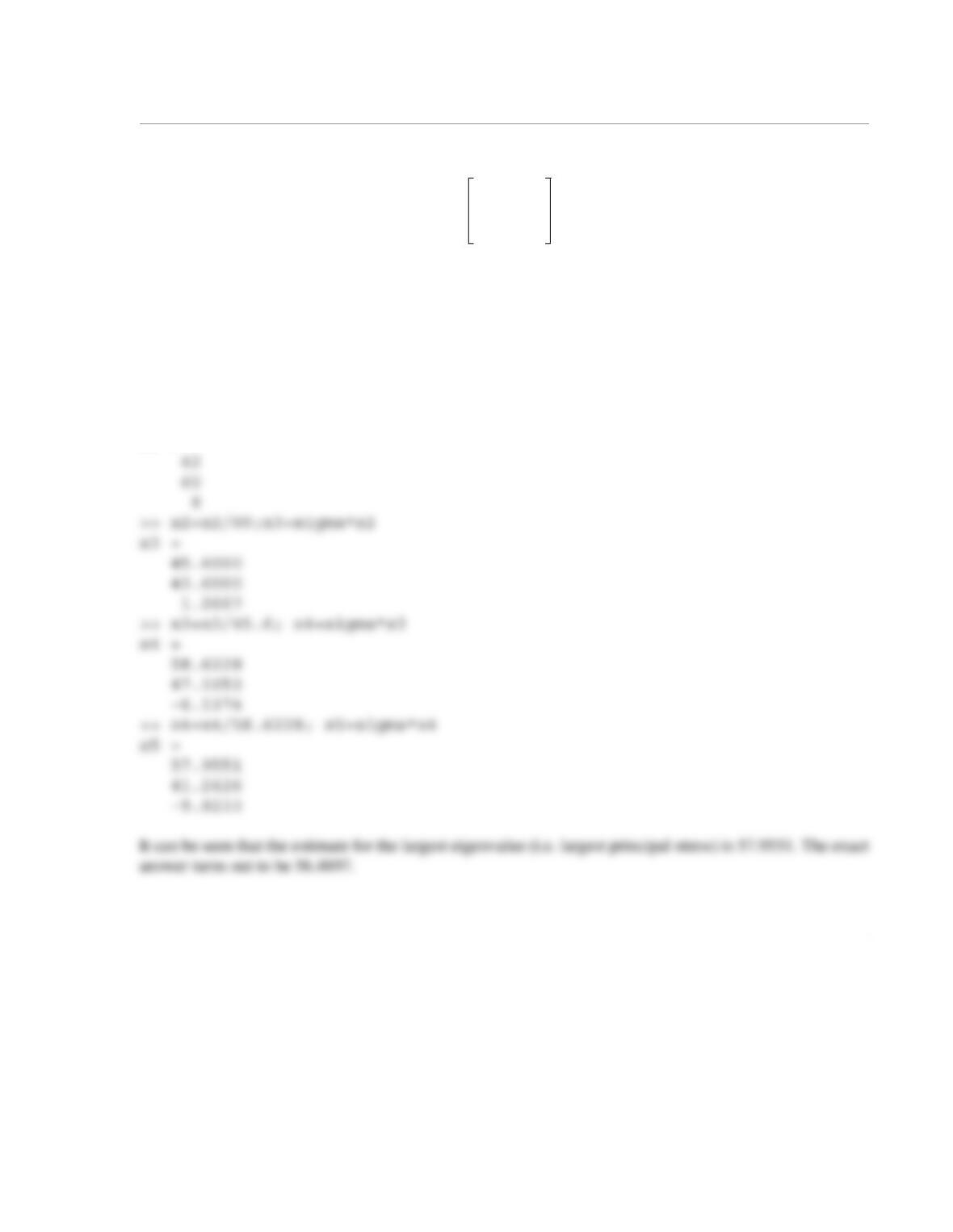
The calculations are carried out in the MATLAB command window:
>> >> A=[1 1 2; 4 1 5; 0 0 1];
>> x1=[1;1;1]; x2=A*x1
x2 =
4
10
1
1
5.8 The three-dimensional state of stress at a point is given by the stress tensor:
ksi
The principal stresses and the principal directions at the point are given by the eigenvalues and the eigen-
vectors. Use the power method for determining the value of the largest principal stress. Start with a column
vector of 1s, and carry out the first three iterations.
Solution
The calculations are carried out in the MATLAB command window:
>> sigma=[40 20 -18; 20 28 12; -18 12 14];
>> x1=[1;1;1]; x2=sigma*x1
x2 =
σij
40 20 18–
20 28 12
18–1214
=
1
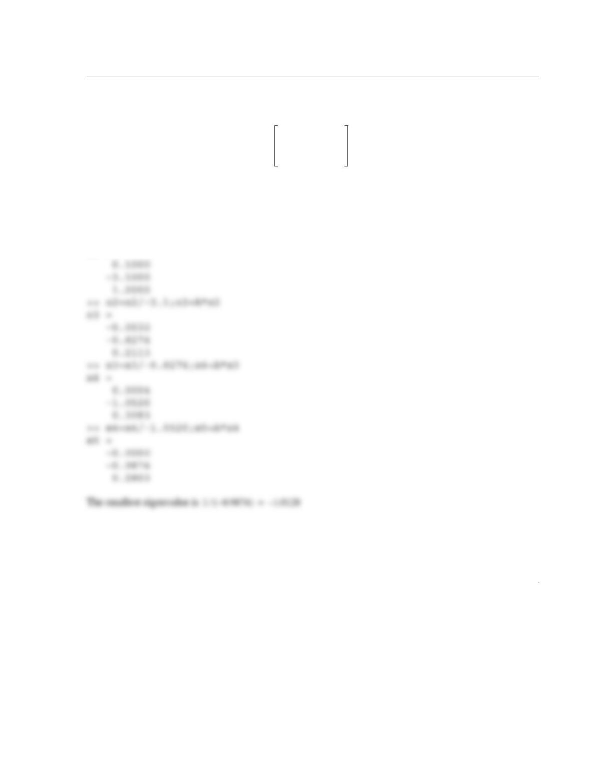
5.9 Apply the inverse power method to find the smallest eigenvalue of the matrix from Problem 5.3
starting with the vector [1 1 1]T. The inverse of the matrix in Problem 5.3 is:
Solution
The calculations are carried out in the MATLAB command window:
>> A=[0.1 0 0; 0.15 -1.5 -1.75; -0.05 0.5 0.75];
>> x1=[1;1;1]; x2=A*x1
x2 =
0.1 0 0
0.15 1.5–1.75–
0.05– 0.5 0.75
1
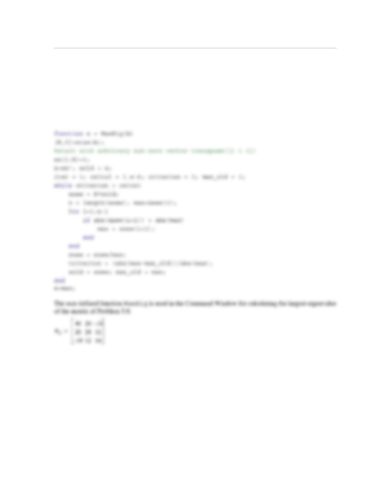
5.10 Write a user-defined MATLAB function that determines the largest eigenvalue of an matrix
by using the power method. For the function name and argument use e = MaxEig(A), where A is the
matrix and e is the value of the largest eigenvalue. Use the function MaxEig for calculating the largest
eigenvalue of the matrix of Problem 5.8. Check the answer by using MATLAB’s built-in function for find-
ing the eigenvalues of a matrix.
Solution
The listing of the user-defined function MaxEig is:
nn×()