Chapter 3 Homework For Nickel Which Sometimes Used Such Detectors

1

3.23 Modify the function NewtonRoot that is listed in Fig. 3-11, such that the output will have three

arguments. Name the function

[

Xs,FXs,iact]

=

NewtonRootMod

(

Fun,FunDer,Xest,Err,imax

)

. The

first output argument is the solution, the second is the value of the function at the solution, and the third is

the actual number of iterations that are performed to obtain the solution. Use the function

NewtonRootMod

to solve the equation that is solved in Example 3-2.

Solution

function [Xs,FXs,iact] = NewtonRootMod(Fun,FunDer,Xest,Err,imax)

% NewtonRoot finds the root of Fun = 0 near the point Xest using Newton’s

method.

2

end

if i == imax

fprintf(‘Solution was not obtained in %i iterations.\n’,imax)

Xs = (‘No answer’);

end

To solve the equation in Example 3-2, the following user-defined functions that calculate

and

are created.

fx() 84.5xxsin–()–=

f′x() 4.5 1 xcos–()–=

3.24 Steffensen’s method is a scheme for finding a numerical solution of an equation of the form

that is similar to Newton’s method but does not require the derivative of . The solution pro-

cess starts by choosing a point , near the solution, as the first estimate of the solution. The next estimates

of the solution are calculated by:

Write a MATLAB user-defined function that solves a nonlinear equation with Steffensen’s method. Name

the function Xs = SteffensenRoot(Fun,

Xest

), where the output argument Xs is the numerical solu-

tion. The input argument Fun is a name for the function that calculates for a given x (it is a dummy

name for the function that is imported into SteffensenRoot), and

Xest

is the initial estimate of the

solution. The iterations should stop when the estimated relative error (Eq. (3.9)) is smaller than . The

number of iterations should be limited to 100 (to avoid an infinite loop). If a solution with the required

accuracy is not obtained in 100 iterations, the program should stop and display an error message.

Use the function SteffensenRoot to solve Problems 3.2 and 3.3.

Solution

function Xs = SteffensenRoot(Fun,Xest)

% SteffensenRoot finds the root of Fun = 0 near the point Xest using

Steffensen’s method.

% Input variables:

fx() 0=

fx()

xi

xi1+

xi1+ xi

fx

i

()

2

fx

ifx

i

()+()fx

i

()–

—————-—————-————–

–=

fx()

10 6–

2

end

if i == imax

fprintf(‘Solution was not obtained in %i iterations.\n’,imax)

Xs = (‘No answer’);

end

Script file that solves Problems 3.2 and 3.3:

1

3.25 Write a user-defined MATLAB function that solves for all the real roots in a specified domain of a

nonlinear function using the bisection method. Name the function R=BisecAll-

Roots(fun,a,b,TolMax). The output argument R is a vector whose elements are the values of the

roots. The input argument Fun is a name for a function that calculates for a given x. (It is a dummy

name for the function that is imported into BisecAllRoots.) The arguments a and b define the domain,

and TolMax is the maximum tolerance that is used by the bisection method when the value of each root is

calculated. Use the following algorithm:

1. Divide the domain into 10 equal subintervals of length h such that .

2. Check for a sign change of at the endpoints of each subinterval.

3. If a sign change is identified in a subinterval, use the bisection method for determining the root in that

subinterval.

4. Divide the domain into 100 equal subintervals of length h such that .

5. Repeat step 2. If a sign change is identified in a subinterval, check if it contains a root that was already

obtained. If not, use the bisection method for determining the root in that subinterval.

6. If no new roots have been identified, stop the program.

7. If one or more new roots have been identified, repeat steps 4–6, wherein each repetition the number of

subintervals is multiplied by 10.

Use the function BisecAllRoots, with TolMax value of 0.0001, to find all the roots of the equa-

tion .

Solution

function R = BisecAllRoots(Fun,a,b,TolMax)

% BisecAllRoot finds all the roots of Fun = 0 in the interval [a,b]

fx() 0=

fx()

ab,[]

hba–()10⁄=

fx()

ab,[]

hba–()100⁄=

x45.5x3

–7.2x2

–43x36++ 0=

2

j = 0;

while c==1

c = 0;

Fbi = Fun(bi);

% Cgecking for a sign change in a subinterval.

if Fai*Fbi < 0 %If a sign change is detected, calculate the root.

xs=BisectionRoot(Fun,ai,bi,TolMax);

% Assign the root to vector R.

if n==10 & is==1

R(is)=xs;

is=is+1;

3

end

n = 10*n; % Increase the number of subitervals by a factor of 10.

end

To find the roots of the equation the following user-defined function is

created.

x45.5x3

–7.2x2

–43x36++ 0=

1

3.26 Examine the differences between the True Relative Error, Eq. (3.8), and the Estimated Relative

Error, Eq. (3.9), by numerically solving the equation . The exact solution of the

equation is . Write a MATLAB program in a script file that solves the equation by using

Newton’s method. Start the iterations at , and execute 11 iterations. In each iteration, calculate the

True Relative Error (TRE) and the Estimated Relative Error (ERE). Display the results in a four-column

table (create a 2-dimensional array), with the number of iterations in the first column, the estimated numer–

ical solution in the second, and TRE and ERE in the third and fourth columns, respectively.

Solution

Script file:

clear all

F=@ (x) 0.5*exp(2+x)-40;

FD=@ (x) 0.5*exp(2+x);

When the script file is executed, the display in the Command Window is:

Exact solution 2.38202663467e+000

Iteration Num Sol TRE ERE

1 3.19830017413e+000 -3.42680273838e-001 -2.00424956467e-001

fx() 0.5e2x+()

40–0==

x80()ln 2–=

x4=

2

1

3.27 When calculating the payment of a mortgage, the relationship between the loan amount, Loan, the

monthly payment, MPay, the duration of the loan in months Months, and the annual interest rate, Rate, is

given by the equation (annuity equation):

Determine the rate of a 20 years, $300,000 loan if the monthly payment is $1684.57.

(a) Use the user-defined function SteffensenRoot from Problem 3.24.

(b) Use MATLAB’s built-in function fzero.

Solution

(a) The function is: , which can be written as:

.

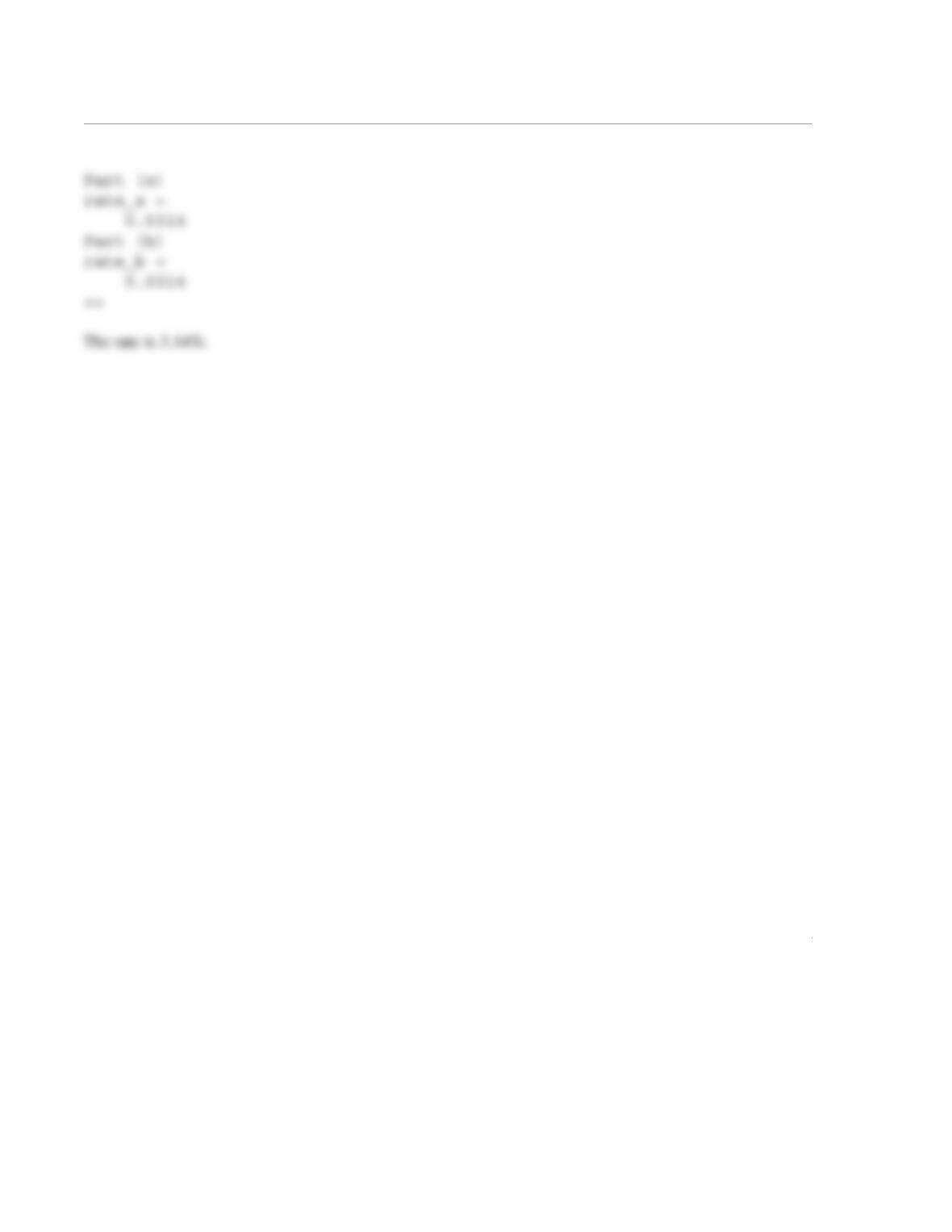
A plot of the function (shown on the right) for the domain is obtained with MATLAB by typing:

MPay Loan Rate⋅

12 11

1Rate

12

———––

+





Months

——————-———————–

–







——————-———————————-———––

=

fx() 1684.57 12 1 1

1x

12

—––

+





12 20⋅

——————————-–

–







⋅300000 x⋅()–=

0.02 0.05,[]

2

1

3.28 The operation of Resistance Temperature Detector (RTD) is based on the fact that the electrical resis-

tance of the detector material changes with temperature. For Nickel which is sometimes used in such

detectors, the resistance, , at temperature T ( ) as a function of temperature is given by:

where is the resistance of the detector at 0 and , ,

, and are constants. Consider a detector with and determine

the temperature when its resistance is 300 .

(a) Use the user-defined function

NewtonSol

given in Problem 3.22.

(b) Use MATLAB’s built-in fzero function.

Solution

The solution is the zero of the function:

RT

°C

RTR01AT BT 2CT 4DT 6

++ + +()=

R0

°C

A5.485 10 3–

×=

B6.65 10 6–

×=

C2.805 10 11–

×=

D2–10

17–

×=

R0100Ω=

Ω

fR() R01AT BT 2CT 4DT 6

++ + +()300–=

2

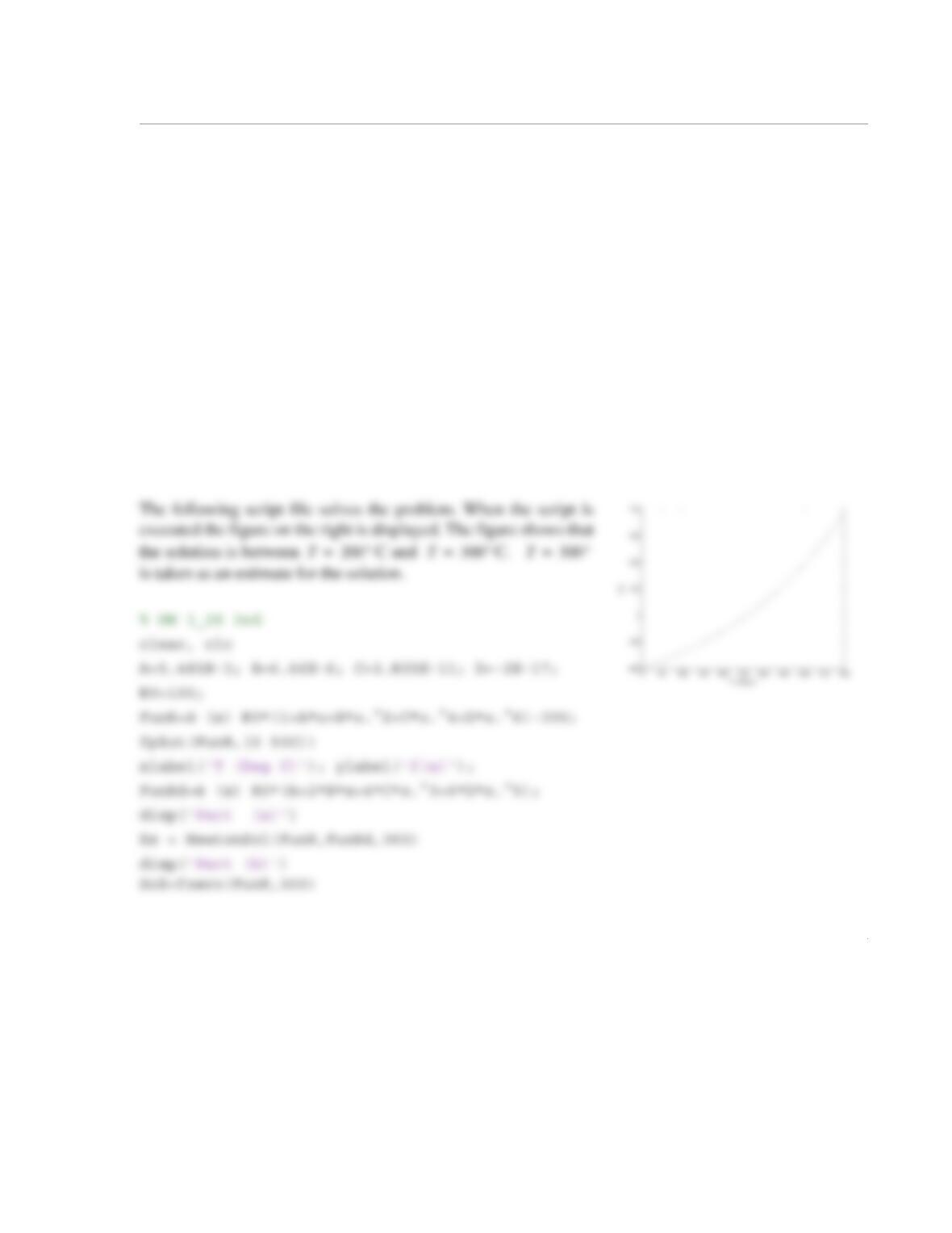
When the script file is executed the following solution is displayed in the Command Window:

Part (a)

Sol_a =

260.1559

1

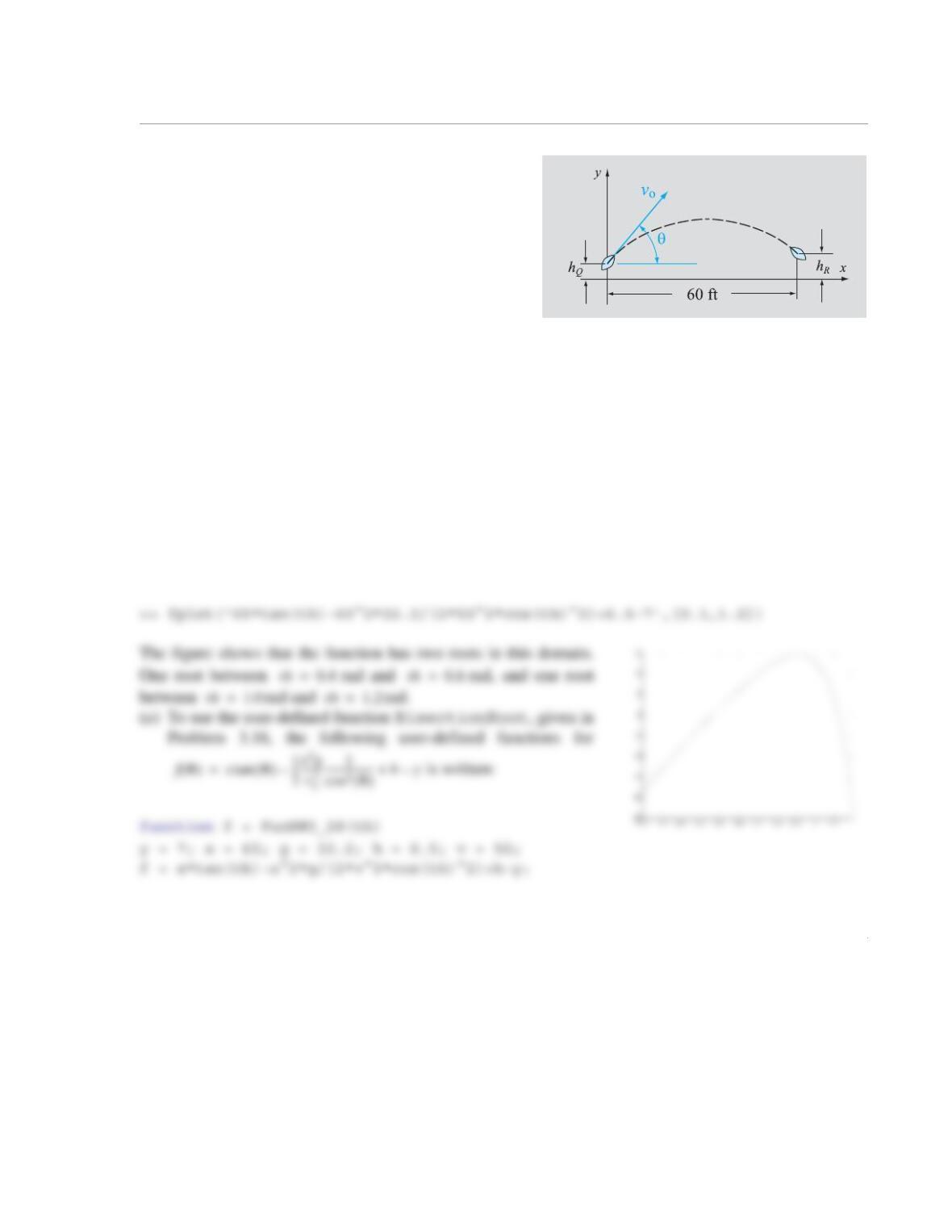
3.29 A quarterback throws a pass to his wide receiver

running a route. The quarterback releases the ball at a

height of . The wide receiver is supposed to catch the

ball straight down the field 60 ft away at a height of .

The equation that describes the motion of the football is

the familiar equation of projectile motion from physics:

where x and y are the horizontal and vertical distance, respectively, ft/s2 is the acceleration due to

gravity, is the initial velocity of the football as it leaves the quarterback’s hand, and θ is the angle the

football makes with the horizontal just as it leaves the quarterback’s throwing hand. For ft/s,

ft, ft, and ft, find the angle θ at which the quarterback must launch the ball.

(a) Use the user-defined function BisectionRoot that was developed in Problem 3.16.

(b) Use MATLAB built-in function fzero.

Solution

The solution is the root of the function .

A plot of the function (shown on the right) for the domain is obtained with MATLAB by typing:

hQ

hR

yx θ()tan 1

2

—–x2g

vo

2

——-–1

θ()cos2

——————–

–hQ

+=

g32.2=

vo

vo50=

x60=

hQ6.5=

hR7=

fθ() xθ()tan 1

2

—–x2g

vo

2

——-–1

θ()cos2

——————–

–hQ7–+=

0.1 1.2,[]

2

(a) In the Command Window, the user-defined function BisectionRoot is then used for finding the

roots. The first root:

>> Xs = BisectionRoot(@FunHW3_29,0.4,0.6)

Xs =

0.4524

1

3.30 The van der Waals equation gives a relationship between the pressure P (in atm.), volume V (in L),

and temperature T (in K) for a real gas:

where n is the number of moles, (L atm)/(mole K) is the gas constant, and a (in L2 atm/mole2)

and b (in L/mole) are material constants.

Consider 1.5 moles of nitrogen ( L2atm/mole2, L/mole) at C stored in a

pressure vessel. Determine the volume of the vessel if the pressure is 13.5 atm.

(a) Use the user-defined function BisectionRoot given in Problem 3.16. Use 0.0001 for TolMax.

(b) Use the user-defined function SecantRoot given in Program 3-3. Use 0.0001 for Err.

(c) Use MATLAB’s built-in fzero function.

Solution

The solution is the root of the function .

A plot of the function (shown on the right) for the domain is obtained with MATLAB by typing:

PnRT

Vb–

———–– n2a

V2

——-–

–=

R0.08206=

a1.39=

b0.03913=

25°

fV() nRT

Vb–

———–– n2a

V2

——-–

–P–=

15,[]

2

>> Xs = BisectionRoot(@FunHW3_30,2,3)

Xs =

2.6707

(b) The user-defined function SecantRoot given in Program 3-3 is used with , ,

0.0001 for Err., and imax 30.

Xa 2=

Xb 3=

1

3.31 The force F acting between a particle with a charge q and a round disk with a radius R and a charge

Q is given by the equation:

where C2/(Nm2) is the permittivity constant and z is the distance to the particle. Deter–

mine the distance z if N, C, and C, and m.

(a) Use the user-defined function BisectionRoot that was developed in Problem 3.16 with a starting

interval of .

(b) Use the user-defined function SteffensenRoot from Problem 3.24.

(c) Use MATLAB’s built-in function fzero.

Solution

The solution is the zero of the function:

FQqz

2ε0

———–1z

z2R2

+

—————–—–

–





=

ε00.885 10 12–

×=

F0.3=

Q9.4 10 6–

×=

q2.4 10 5–

×=

R0.1=

0.1 0.2,[]

-0.05

0

0.05

0.1

0.15

f(z)

fz() Qqz

2ε0

———–1z

z2R2

+

——————-––

–





0.3–=

2

z_b = SteffensenRoot(Fun,0.2)

disp(‘Part (c)’)

z_c=fzero(Fun,0.2)

The following is displayed in the Command Window when the script is executed:

1

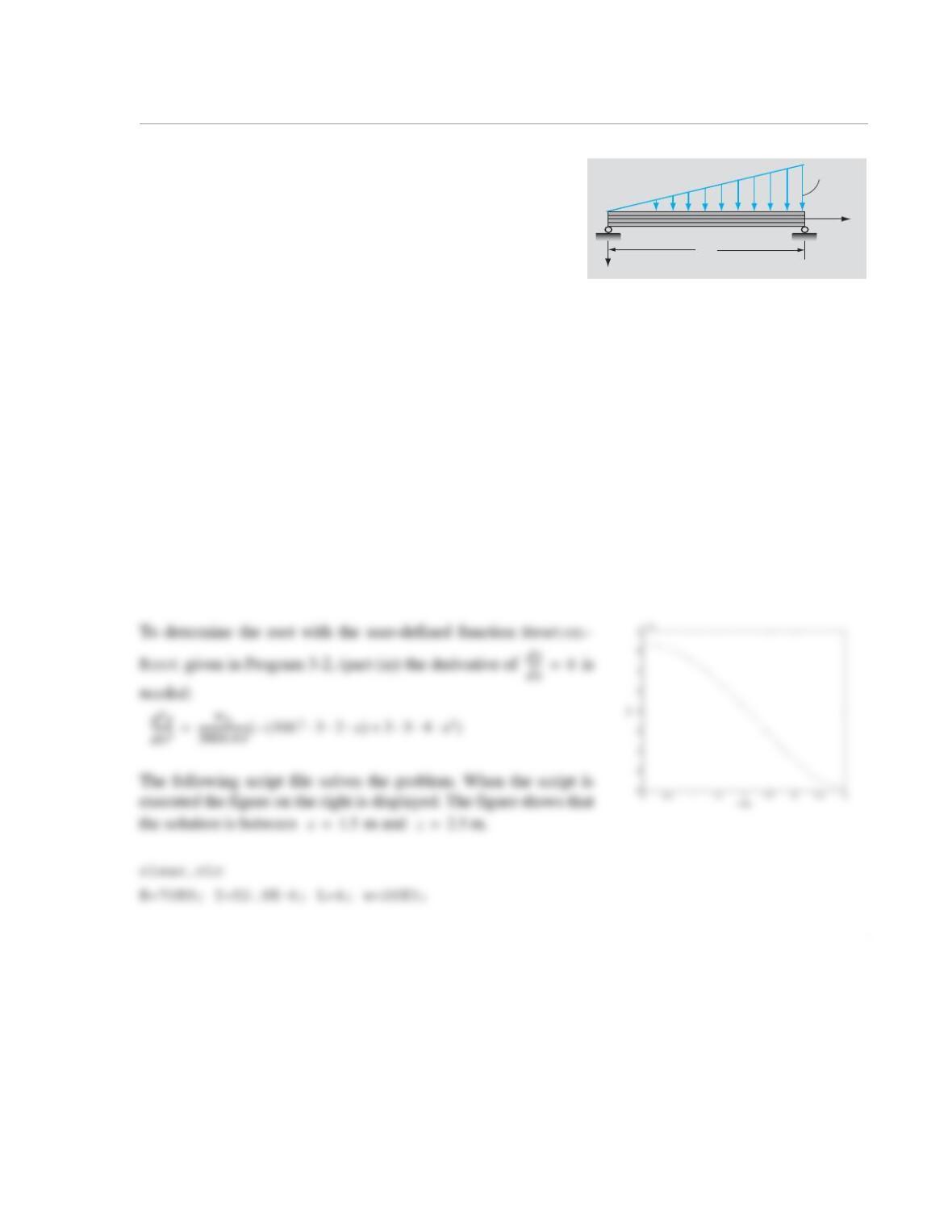
3.32 A simply supported I-beam is loaded with a distributed

load, as shown. The deflection, y, of the center line of the beam

as a function of the position, x, is given by the equation:

where m is the length, GPa is the elastic modu-

lus, m4 is the moment of inertia, and

kN/m.

Find the position x where the deflection of the beam is maximum, and determine the deflection at

this point. (The maximum deflection is at the point where .)

(a) Use the user-defined function

NewtonSol

given in Problem 3.22.

(b) Use the user-defined function SecantRoot given in Program 3-3. Use 0.0001 for Err, 1.5 for Xa.

and 2.5 for Xb.

(c) Use MATLAB’s built-in fzero function.

Solution

The deflection of the beam is maximum at the point where .

x

yL

w

0

yw0x

360LEI

——————–7L410L2x2

–3x4

+()=

L4=

E70=

I52.9 10 6–

×=

w020=

dy

dx

—––0=

dy

dx

—––0=

dy

dx

—––w0

360LEI

——————–7L410L23x2

⋅⋅()–35x4

⋅⋅+()=