Chapter 6 Homework it is only necessary to calculate the linear spline between

1

6.14 Determine the fourth-order Newt on’s interpolating polynomial that passes through the data poi nts

given in Problem 6.13. Use the polynomial to calculate the power at a wind speed of 26 mph.

Solution

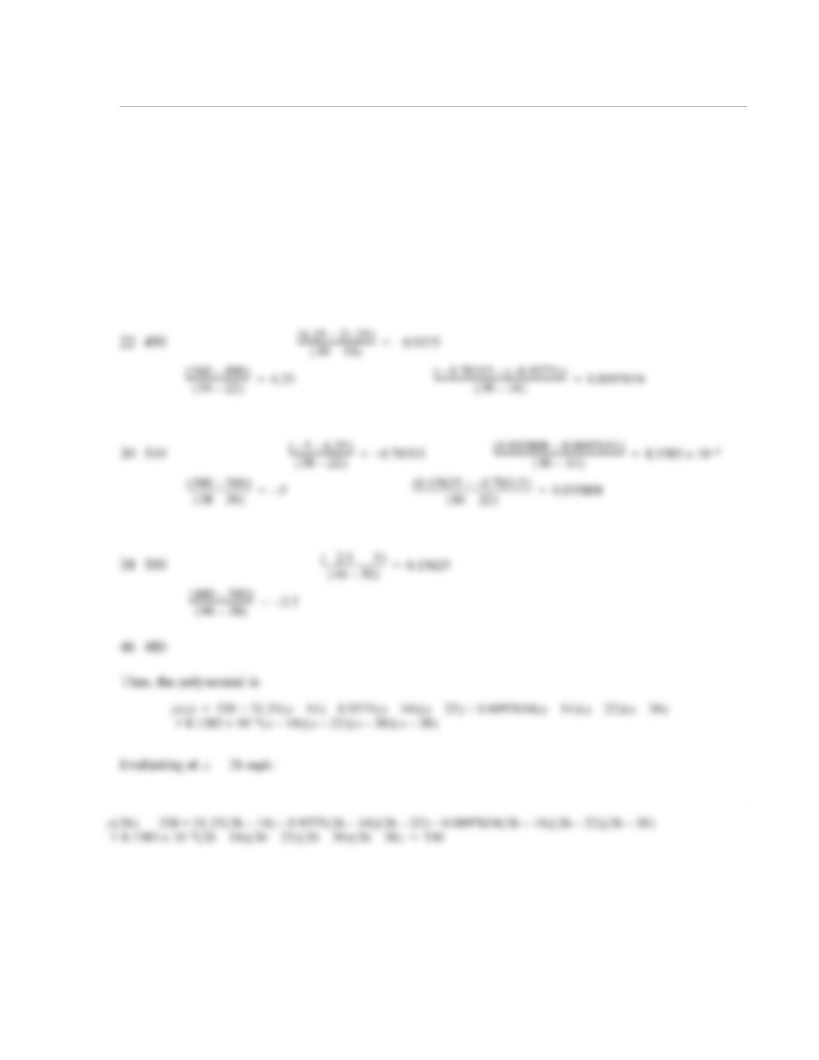
Write the data in column form as follows, and use the method of divided differences:

x y

14 320

490 320–()

22 14–()

—————–———-– 21.25=

1

6.15 The following data is given:

(a) Write the polynomial in Lagrange form that passes through the points; then use it to calculate the inter–

polated value of y at .

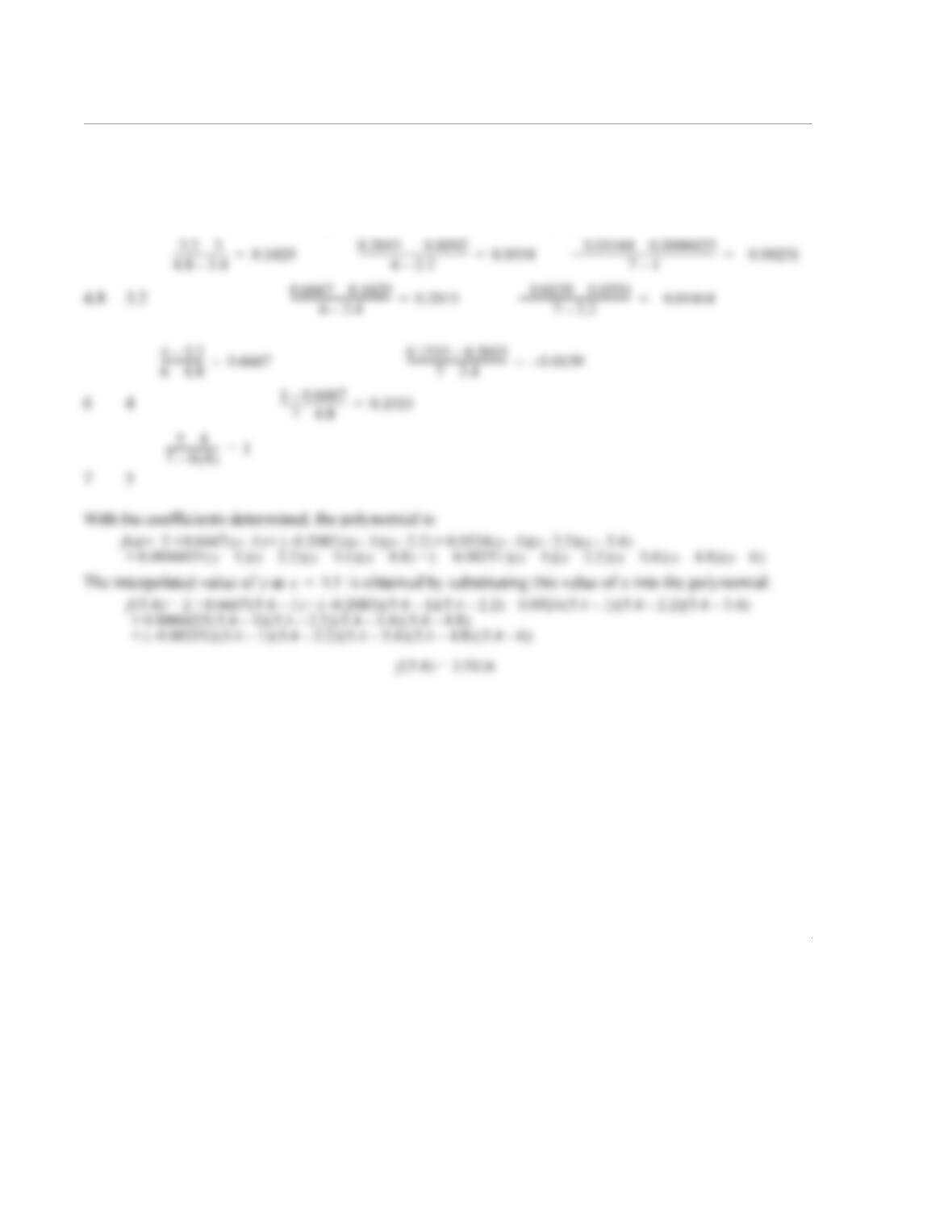
(b) Write the polynomial in Newton’s form that passes through the points; then use it to calculate the inter–

polated value of y at .

Solution

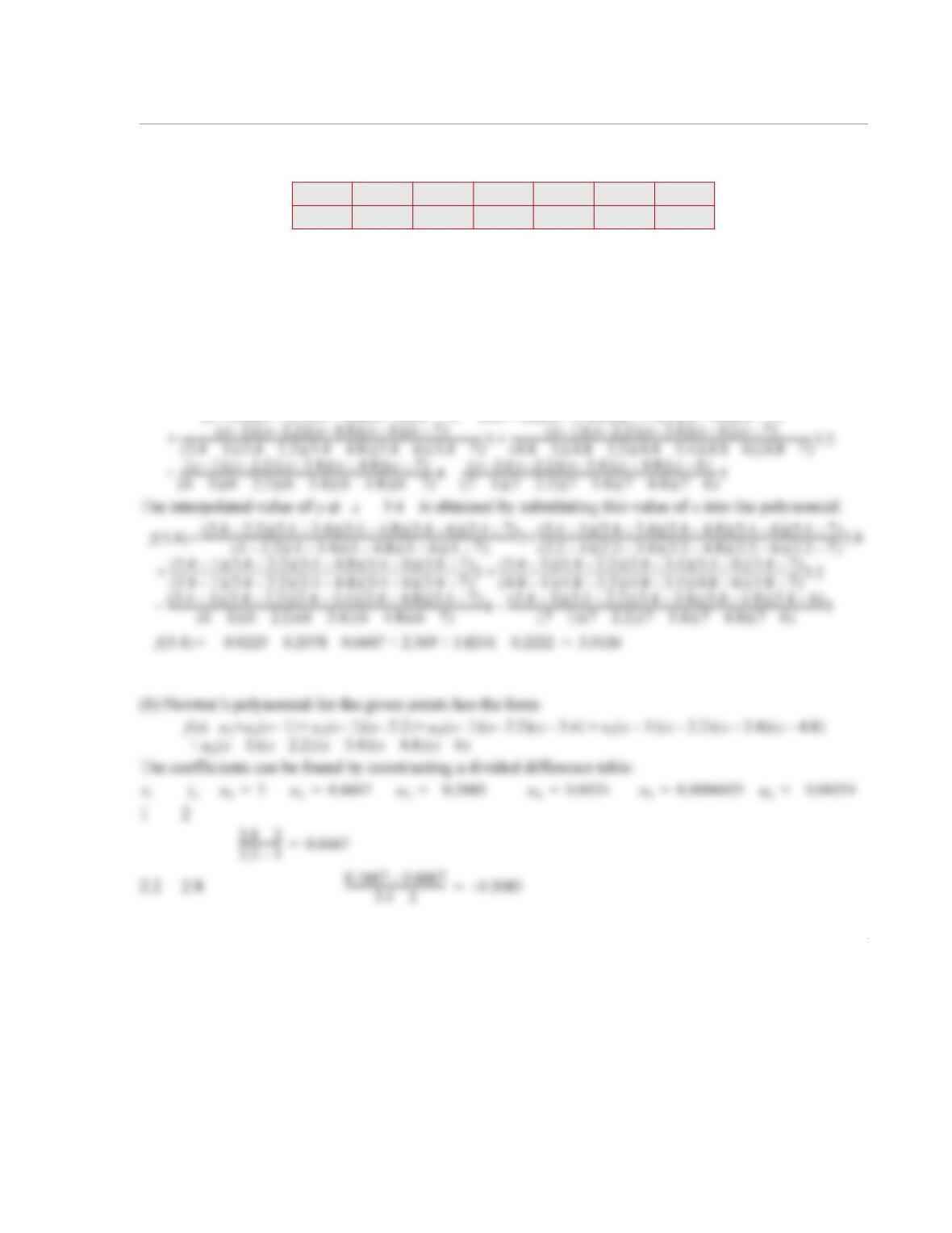
(a) Following the form of Eq. (5.44), the Lagrange polynomial for the six given data points is:

x12.2 3.4 4.8 6 7

y22.8 33.2 4 5

x5.4=

fx() x2.2–()x3.4–()x4.8–()x6–()x7–()

12.2–()13.4–()14.8–()16–()17–()

—————-———————————-———————————-————––2x1–()x3.4–()x4.8–()x6–()x7–()

2.2 1–()2.2 3.4–()2.2 4.8–()2.2 6–()2.2 7–()

—————————————————-———————————-——————-———––2.8

+

=

2

3.4 3

32.8–

3.4 2.2–

—————-—-–0.1667=

0.0092– 0.2083––

4.8 1–

——————-————————–– 0.0524=

0.1429 0.1667–

4.8 2.2–

—————–—————-—––0.0092–=

0.0554 0.0524–

61–

————————————––0.0006025=

1

6.16 Use linear splines interpolation with the data in Problem 6.13 to calculate the power at the following

wind speeds.

(a)24 mph (b) 35 mph.

Solution

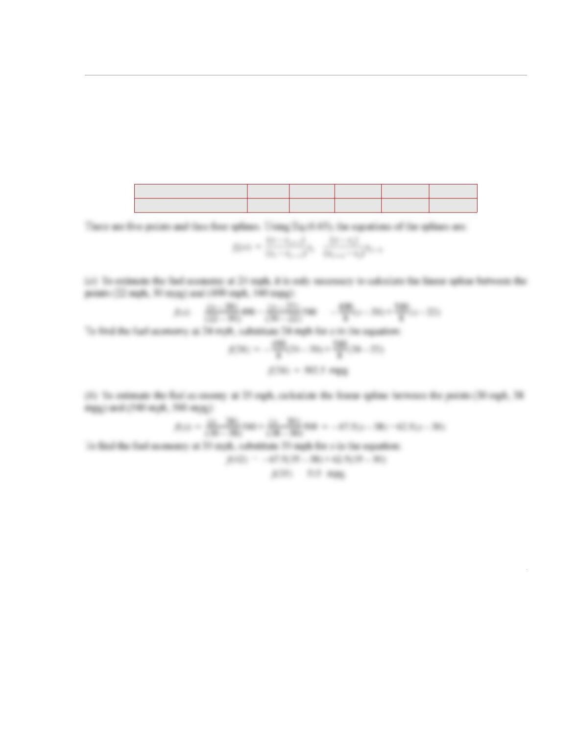
The data in Problem 6.13 is

Wind Speed (mph) 14 22 30 38 46

Electric Power (W) 320 490 540 500 480

1

6.17 Use quadratic splines interpolation with the data in Problem 6.13 to calculate the power at the fol-

lowing wind speeds.

(a)24 mph (b) 35 mph.

Solution

The data in Problem 6.13 is:

Wind Speed (mph) 14 22 30 38 46

Electric Power (W) 320 490 540 500 480

2

This system of equations can be solved using the following MATLAB script:

clear all

A = [14 1 0 0 0 0 0 0 0 0 0; 22 1 0 0 0 0 0 0 0 0 0; 0 0 22^2 22 1 0 0 0 0 0 0

0 0 30^2 30 1 0 0 0 0 0 0; 0 0 0 0 0 30^2 30 1 0 0 0; 0 0 0 0 0 38^2 38 1 0

0 0

When the program is executed, the coefficients are displayed in the Command Window:

c =

1.0e+003 *

0.021250000000000

141 0 00 0 00 0 00

221 0 00 0 00 0 00

0022

222 1 0 0 0 0 0 0

b1

c1

a2

320

490

3

0.000468750000000

The coefficients for the quadratic splines are as follows:

,,,,,, ,,

,,,.

(a) To find the power at 24 mph, consider the polynomial between the points (22 mph, 490 W) and (30

mph, 520 W). This corresponds to , so this polynomial has the coefficients and :

a3b3

,

c3

a10=

b121.25=

c122.5=

a21.875–=

b2103.75=

c2885–=

a30.46875=

b336.875–=

c31224.4=

a40.034722–=

b41.3889=

c4497.36=

i2=

a2b2

,

c2

f2x() 1.875–x2103.75x885–+=

1

6.18 Use natural cubic splines interpolation (based on Lagrange-form polynomials [Eqs. (6.86)–(6.89)])

with the data in Problem 6.13; to calculate the power at the following wind speeds.

(a)24 mph (b) 35 mph.

Solution

The data in Problem 6.13 is:

Wind Speed (mph) 14 22 30 38 46

2

1

6.19 Modify the MATLAB user-defined function LinearRegression in Program 6-1. In addi tion to

determining the constants and , the modified fu nction should also calculate the overa ll error E

according to Eq. (6.6). Name the function [a, Er] = LinReg(x,y). The input arguments x and y are

vectors with the coordinates of the data points. The output argument a is a two-element vector with the val-

ues of the constants and . The output argument Er is the value of the overall error.

(a) Use the function to solve Example 6-1.

(b) Use the function to solve Problem 6.2.

Solution

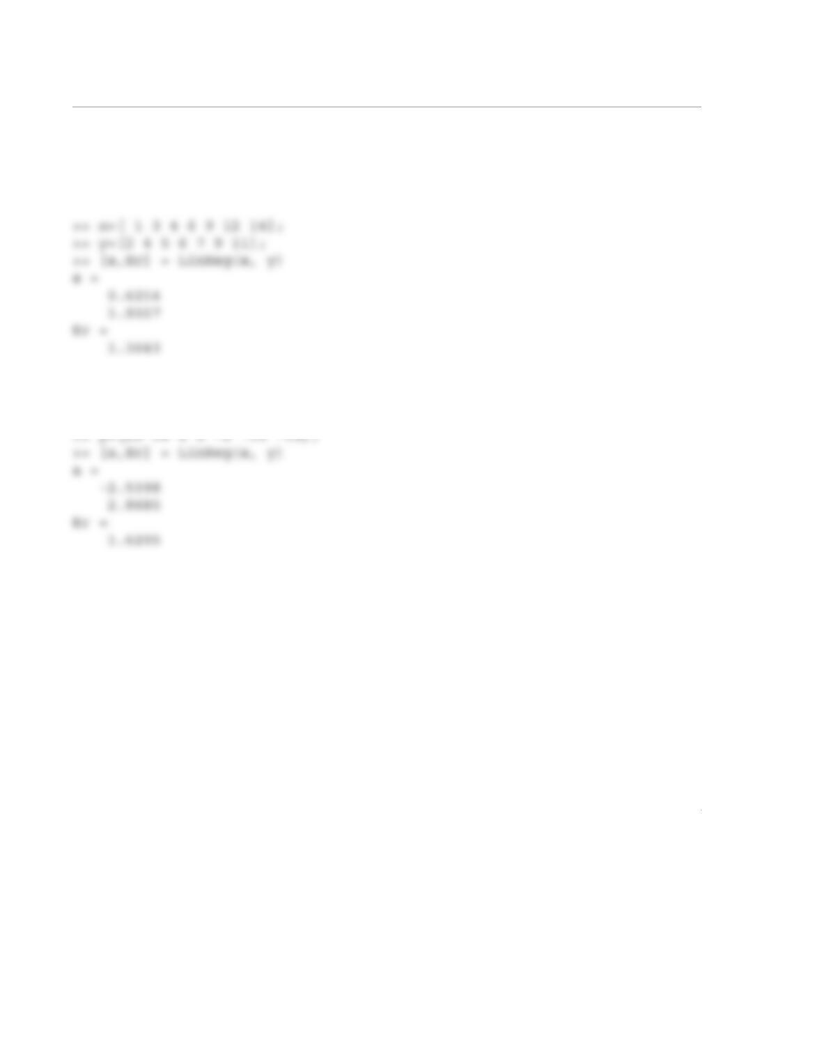
The listing of the user-defined function LinReg is:

function [a,Er] = LinReg(x, y)

% LinReg calculates the coefficients a1 and a0 of the linear

% equation y = a1*x + a0 that best fits n data points, and the overall

a1

a0

a1

a0

2

Er=sum((y-(a1.*x+a0)).^2);

end

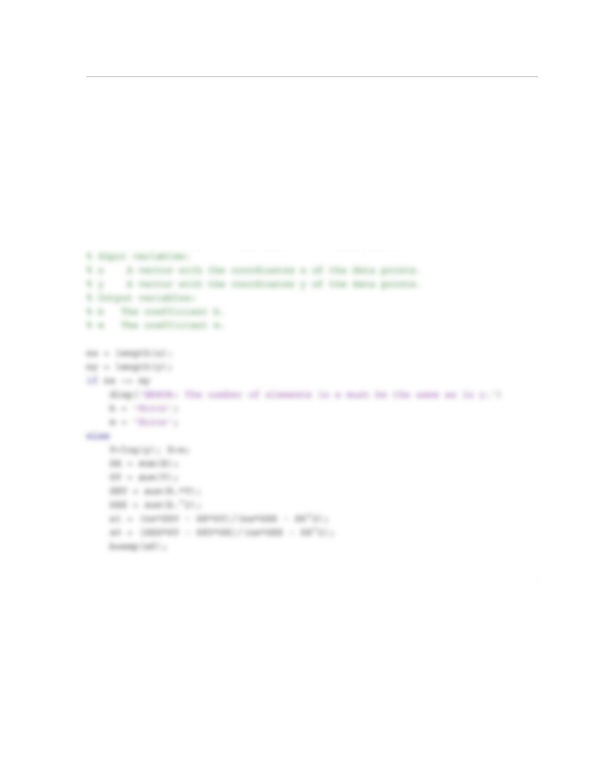
(a) The user-defined function LinReg is used in the Command Window to solve Problem 6.1.

(b) The user-defined function LinReg is used in the Command Window to solve Problem 6.2.

>> x=[-7 -4 -1 0 2 5 7];

1

6.20 Write a MATLAB user-defined function that determines the best fit of an exponential function of the

form to a given set of data points. Name the funct ion [b m]= ExpoFit(x,y), where the

input arguments x and y are vectors with the coordinates of the data points, and the output arguments b

and m are the values of the coefficients. The function ExpoFit should use the approach that is described

in Section 6.3 for determining the value of the coefficients. Use the function to solve Problem 6.8.

Solution

The listing of the user-defined function ExpoFit is:

function [b,m] = ExpoFit(x, y)

% ExpoFit calculates the coefficients b and m of the exponential

% equation y = b*exp(m*x) that best fits n data points.

ybe

mx

=

2

m=a1;

end

The user-defined function ExpoFit is used to solve Problem 6-8 in the following script file:

TC=[-40 -20 0 20 40];

S=[0.0012 0.002 0.0032 0.006 0.0118];

[b,m] = ExpoFit(TC, S)

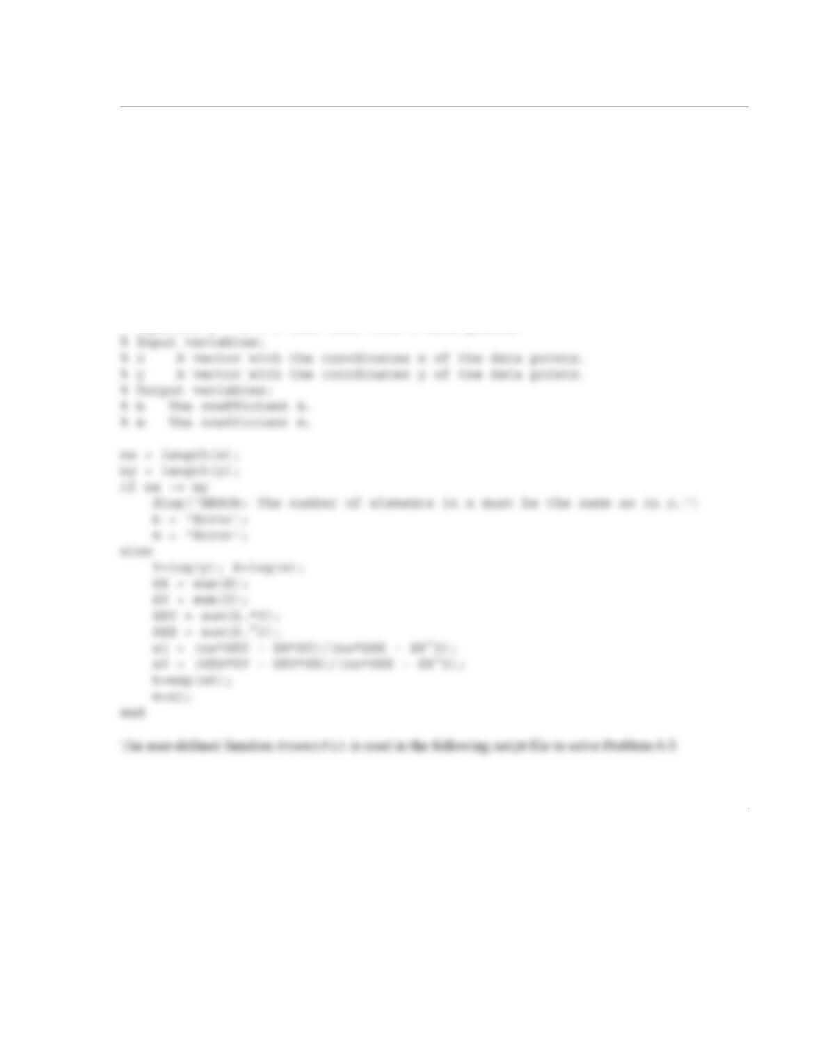
When the script is executed the foll owing answers are displayed in the Command Window, and the following figure

is displayed in the Figure Window.

b =

0.0035

m =

0.0284

1

6.21 Write a MATLAB user-defined function that determines the best fit of a power function of the form

to a given set of data points. Name the function [b m]= PowerFit(x,y), where the input

arguments x and y are vectors with the coordinates of th e data points, and the output arguments b and m

are the values of the coefficients. The function PowerFit should use the approach that is described in

Section 6.3 for determining the value of the coefficients. Use the function to solve Problem 6.3.

Solution

The listing of the user-defined function PowerFit is:

function [b,m] = PowerFit(x, y)

% PowerFit calculates the coefficients b and m of the exponential

% equation y = b*x^m that best fits n data points.

ybx

m

=

2

Y=[1900 1950 1970 1980 1990 2000 2010];

The following results are displayed in the Command Window when the script is executed:

b =

The power function that best fits the data from Problem 5.3 is: .

y7.2065 75–

×10 x23.3944

=

1

6.22 Write a MATLAB user-defined function that determines the coefficients of a quadratic polynomial,

, that best fits a given set of data points. Name the function a = QuadFit(x,y),

where the input arguments x and y are vectors with the coordinates of the data points, and the output argu-

ment a is a three-element vector with the values of the coefficients , and .

(a) Use the function to find the quadratic polynomial that best fits the data in Example 6-2.

(b) Write a program in a script file that plots the data points and the curve of the quadratic polynomial that

best fits the data.

Solution

The listing of the user-defined function QuadFit is:

function a = QuadFit(x, y)

% QuadFit calculates the coefficients a2,a1 and a0 of the quadratic

fx() a2x2a1xa

0

++=

a2

a1

a0

2

X(1,j)=xsum(j-1);

end

% Rows 2 and 3 of matrix [X] and column vector [Y]

(a) The user-defined function QuadFit is used in the Command Window to find the quadratic polynomial

that best fits the data from Example 6-2:

>> t=[2 4 6 8 10 12 14 16 18 20 22 24 26 28 30];

>> V=[9.7 8.1 6.6 5.1 4.4 3.7 2.8 2.4 2.0 1.6 1.4 1.1 0.85 0.69 0.6];

>> a = QuadFit(t, V)

(b) The following program in a script file plots the data points and the curve of the quadratic polynomial

that best fits the data.

clear all; close all; clc;

3

tt=linspace(t(1),t(n),50);

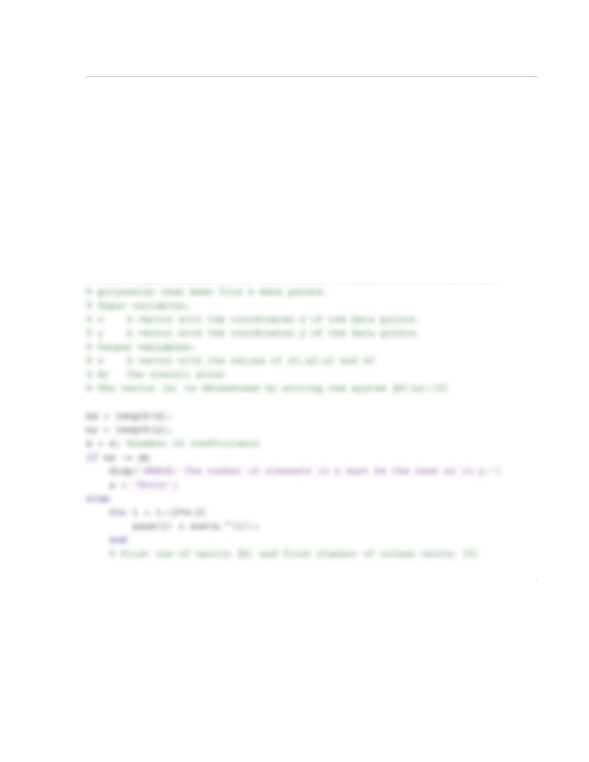
When the program is executed, the following plot is displayed in the Figure Window:

7

8

9

10

Data

Polynomial fit

1

6.23 Write a MATLAB user-defined function that de termines the coefficients of a cubic polynomial,

, that best fits a g iven set of d ata points. The function should al so calculate

the overall error E according to Eq. (6.21). Name the function [a,Er] = CubicPolyFit(x,y), where

the input arguments x and y are vectors with the coordinates of the data points, and the output argument a

is a four-element vector with the values of the coefficients , , , and . The output argument Er is

the value of the overall error.

(a)Use CubicPolyFit to determine the cubic polynomial that best fits the data in Example 6-3.

(b) Write a program in a script file that plots the data points and the curve of the cubic polynomial that best

fits the data.

Solution

The listing of the user-defined function CubicPolyFit is:

function [a,Er] = CubicPolyFit(x, y)

% CubicPolyFit calculates the coefficients a3,a2,a1 and a0 of the cubic

fx() a3x3a2x2a1xa

0

+++=

a3

a2

a1

a0

2

X(1,1) = nx;

Y(1,1) = sum(y);

% Remaining rows of [X] and [Y]

for j = 2:m

X(1,j) = xsum(j – 1);

(a) The user-defined function CubicPolyFit can be used in the Command Window to find the cubic

polynomial that best fits the data from Example 6-3 and the error associated with that polynomial:

>> x=[0 0.4 0.8 1.2 1.6 2 2.4 2.8 3.2 3.6 4 4.4 4.8 5.2 5.6 6];

>> y=[0 3 4.5 5.8 5.9 5.8 6.2 7.4 9.6 15.6 20.7 26.7 31.1 35.6 39.3 41.5];

>> [a,Er] = CubicPolyFit(x,y)

The cubic polynomial which provides the best fit with the data is:

(b) The following program in a script file plots the data points and the curve of the cubic polynomial that

best fits the data.

clear all; close all; clc;

x=[0 0.4 0.8 1.2 1.6 2 2.4 2.8 3.2 3.6 4 4.4 4.8 5.2 5.6 6];

fx() 0.0541–x31.8030x21.9882x– 2.8930++=