3
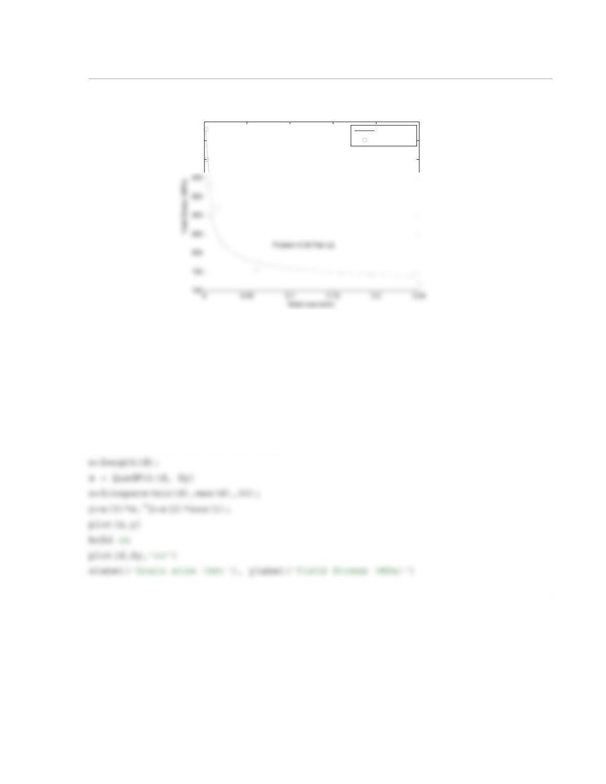
(b) Quadratic function that fits the data has the form:
The following program written in a script file uses the user-defined function QuadFit from Problem 5.20
to find the quadratic function that best fits the data. It also plots the data points and the curve that best fit
the data, and estimates the yield stress for grain size of 0.05 mm.
cclear, clc
d=[0.0018 0.0025 0.004 0.007 0.016 0.06 0.25];
Sy=[530 450 380 300 320 155 115];
450
500
550
Best fit curve
Data points
σya2d2a1da
0
++=
4
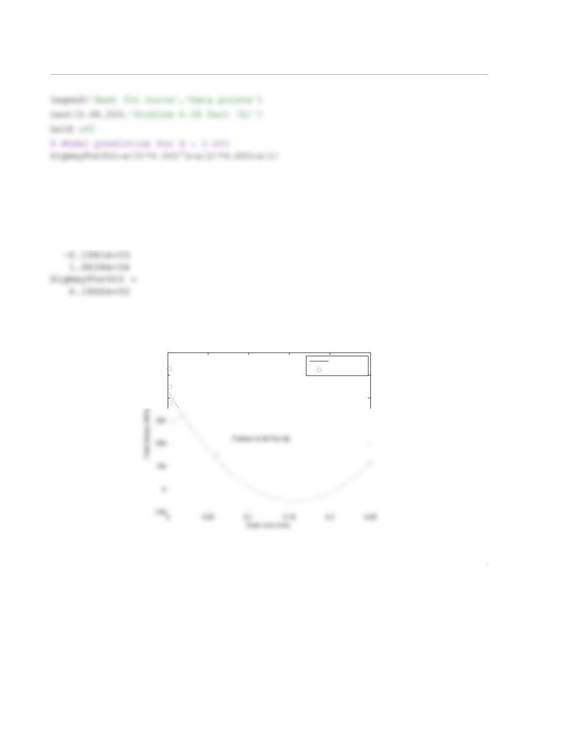
When the program is executed, the values , , and , and the prediction for grain size of 0.05 mm
are displayed in the Command Window. The figure that follows is displayed in the Figure Window.
>> format short e
a =
4.3707e+02
The quadratic equation is:
a0
a1
a2
σy437.07d26194.1d– 19638+=
400
500
600
Best fit curve
Data points
1
6.39 Values of enthalpy per unit mass, h, of an equilibrium Ar gon plasma (Ar, Ar+, A++, A+++ ions and
electrons) versus temperature are:
Write a program in a script file that uses interpolation to calculate h at temperatures ranging from 5000
K to 30000 K in in crements of 500 K. The pro gram should generate a plot that shows the interpolated
points, and the data points from the table (use an asterisk marker).
(a) For interpolation use the user-defined function CubicSplines from Problem 6.24.
(b) For interpolation use MATLAB’s built-in function interp1 with the spline option.
Solution
(a) The following program in a script file solves the problem using the user-defined function Cubic-
Splines from Problem 6.24.
(K) 57.5 10 12.5 15 17.5 20 22.5 25 27.5 30
(MJ/kg) 3.3 7.5 41.8 51.8 61 101.1 132.9 145.5 171.4 225.8 260.9
T103
×
h
2
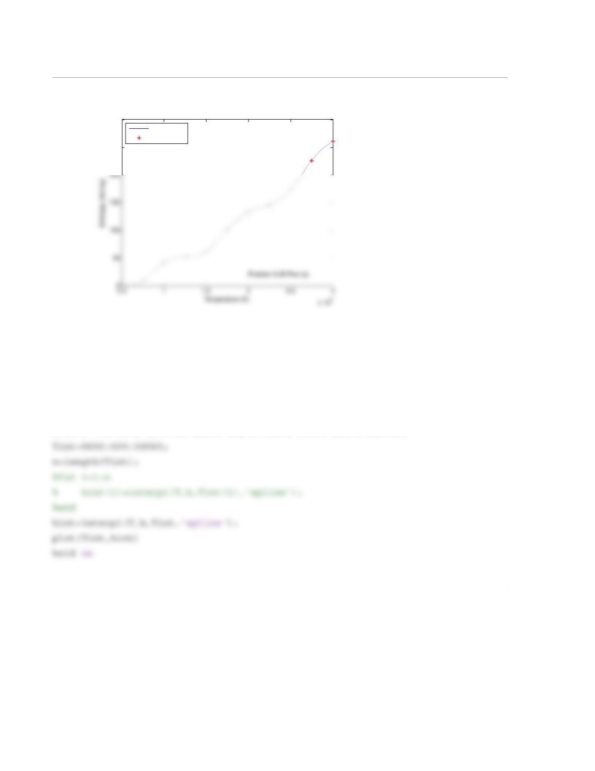
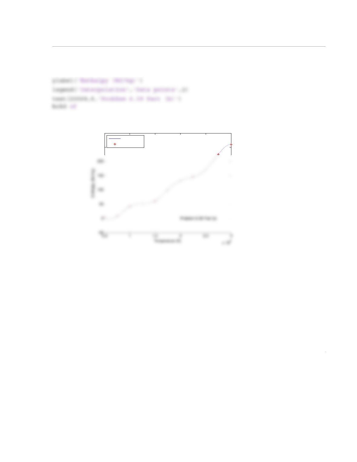
When the script file is executed, the following plot is generated:
(b) The following program in a script file solves the problem using MATLAB’s built-in function
interp1 with the spline option.
clear,clc
T=[5:2.5:30]*1000;
h=[3.3 7.5 41.8 51.8 61 101.1 132.9 145.5 171.4 225.8 260.9];
250
300
Interpolation
Data points
3
plot(T,h,‘*r’)
xlabel(‘Temperature (K)’)
When the script file is executed, the following plot is generated:
250
300
Interpolation
Data points
1
6.40 The following are measurements of the rate coefficient, k, for the reaction at
different temperatures, T:
(a) Use the method of least-squares to bes t fit a function of the form to the data.
Determine the constants C, b, and D by curve fitting a linear combination of the functions ,
, and to the given data (Section 6.8).
(b) Usually, the rate coef ficient is express ed in the form of an Arrhenius equation ,
where A and b are constants, J/mole/K is the universal gas constant, and is the activation
energy for the reaction. Having determined the constants C, b, and D in part (a), deduce the values of A
(m3/s) and (J/mole) in the Arrhenius expression.
Solution
(a) Using Eq. (6.97), the following system of three linear equations for the unknowns C, b, and D can be
written:
T (K) 595 623 761 849 989 1076 1146 1202 1382 1445 1562
(m3/s) 2.12 3.12 14.4 30.6 80.3 131 186 240 489 604 868
CH4O+CH
3OH+→
k10
20
×
k()ln Cb T()ln D
T
—–
–+=
f1T() 1=
f2T() T()ln=
f3T() 1–
T
—––
=
kAT
beEaRT()⁄–
=
R8.314=
Ea
Ea
2
The constants A, b, and are related to the constants C, b, and D that were determined in Part (a) by:
, , and
The computer program calculates the constants and then makes a plot of k versus T. The plot shows the data
points and the line predicted by the equation.
clear, clc
T = [595 623 761 849 989 1076 1146 1202 1382 1445 1562];
k = [2.12 3.12 14.4 30.6 80.3 131 186 240 489 604 868]*1e-20;
n=length(k);
ke
CTbeDT⁄–
=
Ea
Ae
C
=
bb=
DEa
R
—–
=
3
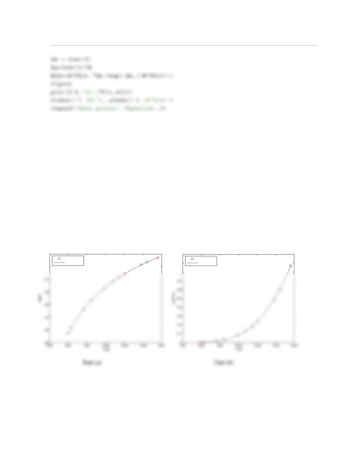
When the program is executed, the values of the constants is displayed in the Command Window, and the
following two figures are displayed.
Command Window:
>> format short e
Cnst =
-5.2443e+001
2.1216e+000
3.8153e+003
A =
1.6765e-023
bb =
2.1216e+000
Ea =
3.1721e+004
−40
−39
Data points
Equation
0.8
0.9
1x 10⁻¹⁷
Data points
Equation
1
6.41 The following measurements were recorded in a study on the growth of trees.
The data is used for deriving an equation that can predict the height of the trees as a function
of their age. Determine which of the nonlinear equations that are listed in Table 6-2 can best fit the data and
determine its coefficients. Make a plot that shows the data points (asterisk marker) and the equation (solid
line).
Solution
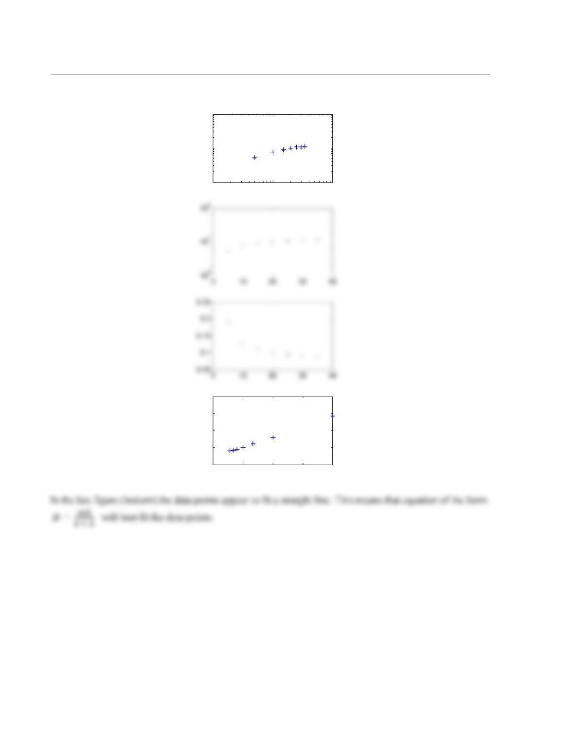
First, the following four plots are made. H (height) vs. A (age) on a log-log plot. H vs. A on a log H (verti-
cal) linear A (horizontal) axes. 1/H vs. A with linear axes. 1/H vs. 1/A with linear axes.
Age (year) 510 15 20 25 30 35
Height (m) 5.2 7.8 910 10.6 10.9 11.2
HHAge()=
2
100101102
100
101
102
00.05 0.1 0.15 0.2
0.05
0.1
0.15
0.2
0.25
3
The constants b and m are then determined by:
clear, clc
p=polyfit(1./A,1./H,1);
Ap=5:0.2:35;
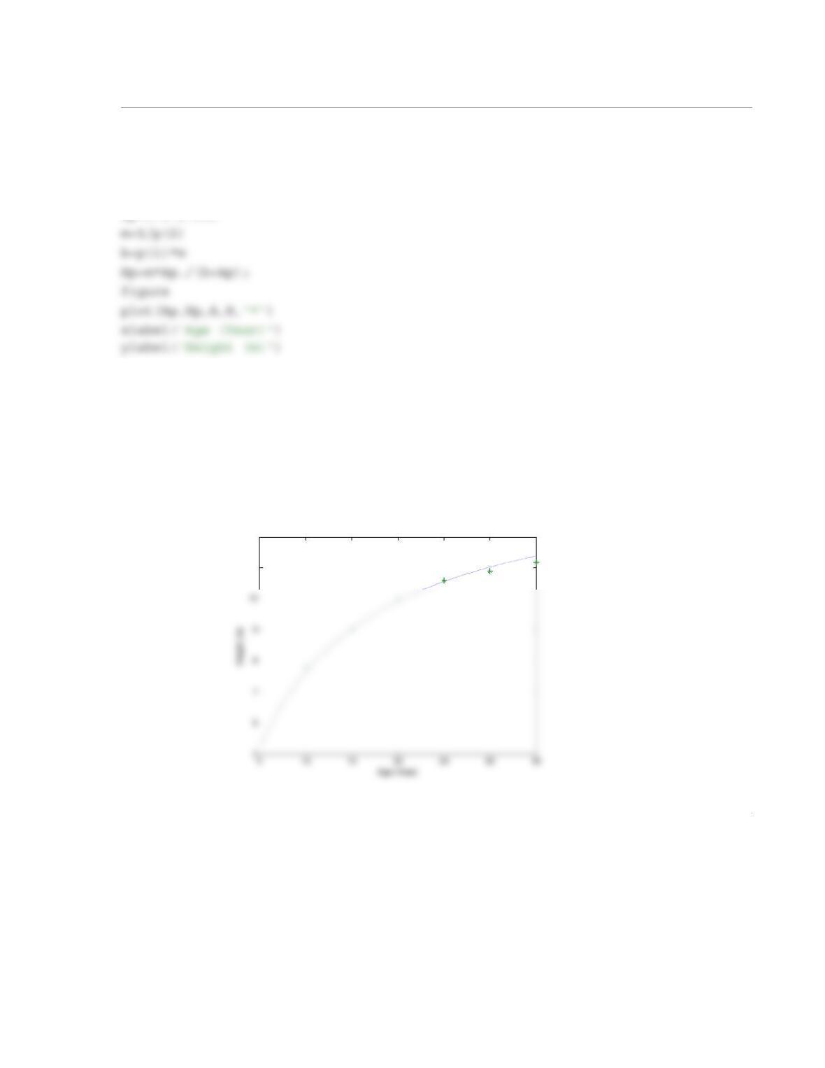
When the script is executed the following values of the constants are displayed in the Command Window,
and the following figure is displayed:
m =
14.1546
b =
8.5285
11
12
1
6.42 The following data present ocean water salinity at different depths:
(a) Use interpolation to estimate the water salinity at depths of 250 m, 750 m, and 1800 m by using the
user-defined function CubicSplines developed in Problem 6.24.
(b) Use interpolation to estimate the water salinity at depths of 250 m, 750 m, and 1800 m by using the
user-defined function CubicLagSplines developed in Problem 6.25.
(c) Use MATLAB to create a vector with values of depth ranging from 0 to 3000 m with spacing of 10 m.
Then use the MATLAB’s built-defined function interp1 with the option spline to calculate corre-
sponding interpolated values of salinity. Make a plot that shows the data points and interpolated points.
Solution
The problem is solved in the following script file:
Depth (m) 0100 200 300 400 500 600 700 800 900 1100 1400 2000 3000
Salinity (ppt) 35.5 35.35 35.06 34.65 34.48 34.39 34.34 34.32 34.33 34.36 34.45 34.58 34.73 34.79
2
S750Partc=interp1(D,S,750,‘spline’)
S51800Partc=interp1(D,S,1800,‘spline’)
DI=linspace(0,3000,100);
SI=interp1(D,S,DI,‘spline’);
plot(DI,SI,D,S,‘*’)
When the script is executed, the fo llowing results are displayed in the Command Window and the figure
that follows is displayed in the Figure Window.
Part (a)
S250Parta =
3.4844e+01
3.4847e+01
S750Partb =
3.4322e+01
S51800Partb =
3.4694e+01
Part (c)
S250Partc =
35
35.2
35.4
35.6
1
6.43 The following data present the power of a diesel engine at different engine speeds:
(a) Estimate the engine power at speeds of 2300 rpm and 3650 rpm by using the user-defined function
CubicSplines developed in Problem 6.24.
(b) Estimate the engine power at speeds of 2300 rpm and 3650 rpm by using the user-defined function
CubicLagSplines developed in Problem 6.25.
(c) Use MATLAB to create a vector with values of engine speeds ranging from 1200 to 4400 rpm with
spacing of 10 rpm. Use the MATLAB’s built-defined function interp1 with the option spline to
calculate corresponding interpolated values of engine power. Make a plot that shows the data points
and interpolated points.
Solution
The problem is solved in the following script file:
clear, clc
S=[1200 1500 2000 2500 3000 3250 3500 3750 4000 4400];
P=[65 130 185 225 255 266 275 272 260 230];
Engine Speed (rpm) 1200 1500 2000 2500 3000 3250 3500 3750 4000 4400
Engine Power (hp) 65 130 185 225 255 266 275 272 260 230
2
ylabel(‘Engine Power (hp)’)
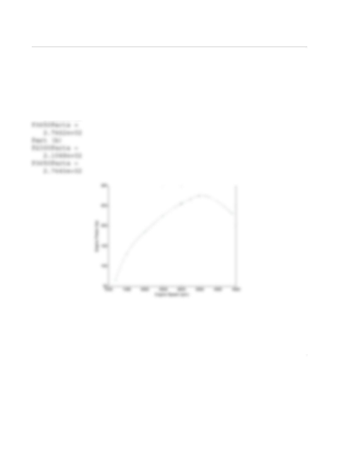
When the script is executed, the fo llowing results are displayed in the Command Window and the figure
that follows is displayed in the Figure Window.
Part (a)
P2300Parta =
2.0950e+02