3
>> format compact
>> x=[0 1 2 3 4];
>> y=[0 1 2 3 4];
>> f=[0 3 14 7 5
8 10 14 12 10
2 7 8 9 7
Note that in the MATLAB script, i is the index used for the variable x and j is the index used for
the variable y. Consequently, the transpose of what is given for the function values in the table in
Problem (6.13) is what has to be input to the program.
1
8.26 Write a MATLAB user-defined function that evaluates the partial second derivatives and
of a function that is specified by discrete tabulated points with equal spacing. Use three-point cen-
tral difference formulas for the interior points and one-sided four-point forward and backward difference
formulas for the end points. For the function name use [dfdx2,dfdy2]= ParDerSnd(x,y,f). The
input arguments x and y are vectors with the values of the independent variables. f is a vector with the
value of f at each point. The output arguments dfdx2 and dfdy2 are vectors with the values of the partial
second derivatives at each point. Use ParDerSnd to calculate the partial second derivatives with respect
to x and y of the function given in Problem 8.14.
Solution
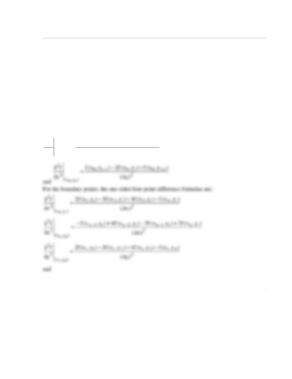
Since the points are equally spaced, we can use the formulae from Table 8-1 in each coordinate
direction. For the interior points, the three-point central difference formulae are:
∂2f
x2
∂
——-–
∂2f
y2
∂
——-–
fxy,()
2
01i0i01i
)y,x(
2
2
)x(
)y,x(f)y,x(f2)y,x(f
x
f
0i Δ
+−
=
∂
∂+−
2
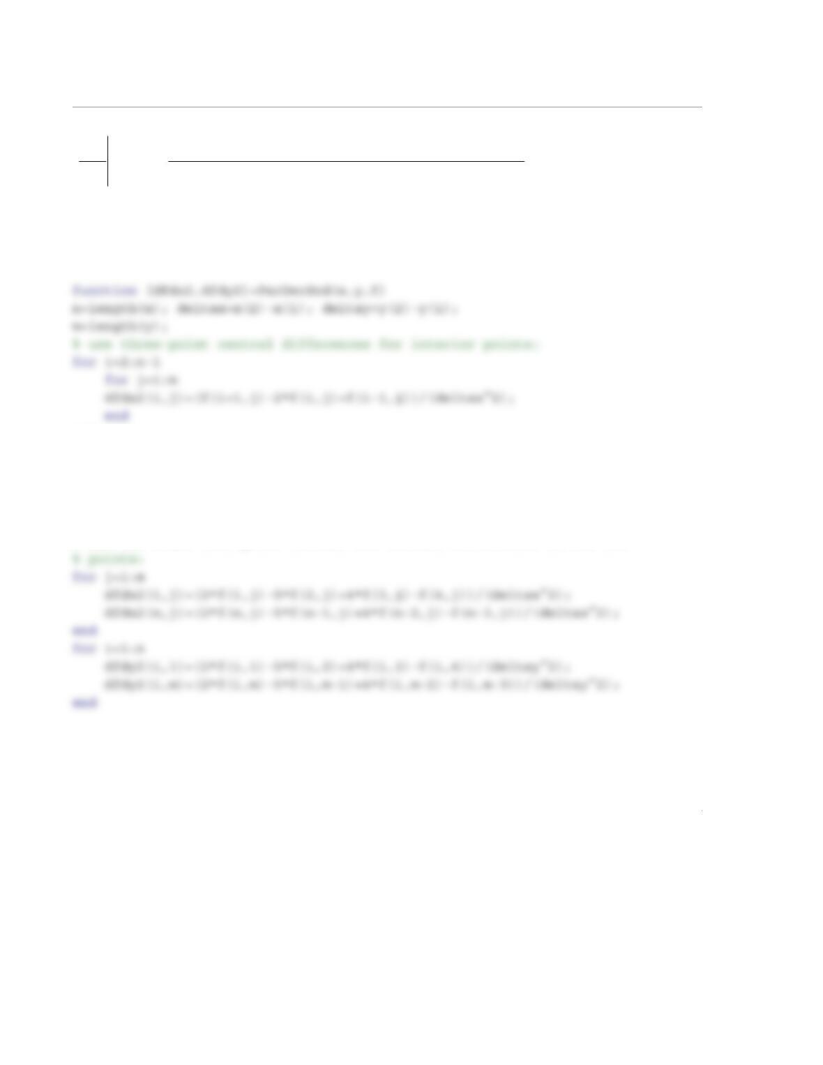
The following user-defined function calculates the partial derivatives according to the above
formulae:
end
for j=2:m-1
for i=1:n
dfdy2(i,j)=(f(i,j+1)-2*f(i,j)+f(i,j-1))/(deltay^2);
end
end
% use one-sided four-point forward and bacward differences at the end
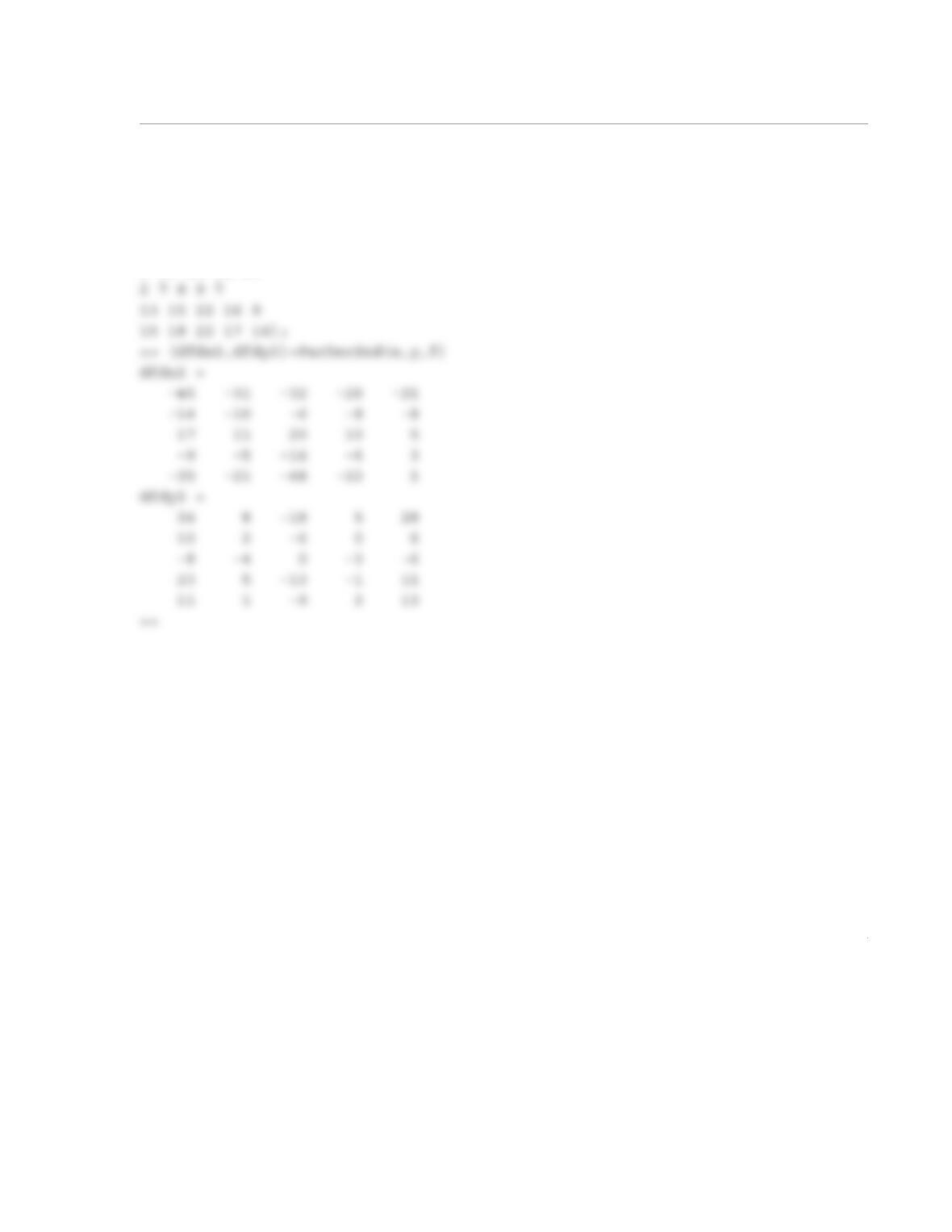
When executed for the function specified in Problem (8.14), the following output is produced:
2
ni1ni2ni3ni
)y,x(
2
2
)y(
)y,x(f2)y,x(f5)y,x(f4)y,x(f
y
f
ni Δ
+−+−
=
∂
∂−−−
3
>> format compact
>> x=[0 1 2 3 4];
>> y=[0 1 2 3 4];
>> f=[0 3 14 7 5
8 10 14 12 10
Note that in the MATLAB script, i is the index used for the variable x and j is the index used for
the variable y. Consequently, the transpose of what is given for the function values in the table in
Problem (8.14) is what has to be input to the program.
1
8.27 The following data is obtained for the velocity of a vehicle during a crash test.:
If the vehicle weight is 2,400 lb, determine the instantaneous force F acting on the vehicle during the crash.
The force can be calculated by , and the mass of the car m is slug.
Note that 1 ms = s and 1 mile = 5,280 ft.
(a) Solve by using the user-defined function FirstDeriv that was written in Problem 8.17.
(b) Solve by the using MATLAB built-in function diff.
Solution
The two parts are solved in the following script file:
clear, clc,
m=2400/32.2;
When the script is executed, the following results are displayed in the Command Window:
Part (a)
Fa =
1.0e+04 *
-0.0000 -1.0932 -3.5528 -9.8385 -9.8385 -4.3727 -2.4596
-1.0932 0
t (ms) 010 20 30 40 50 60 70 80
v (mph) 30 29.5 28 23 10 5 2 0.5 0
Fm
dv
dt
—––
=
2400 32.2⁄
10 3–
1
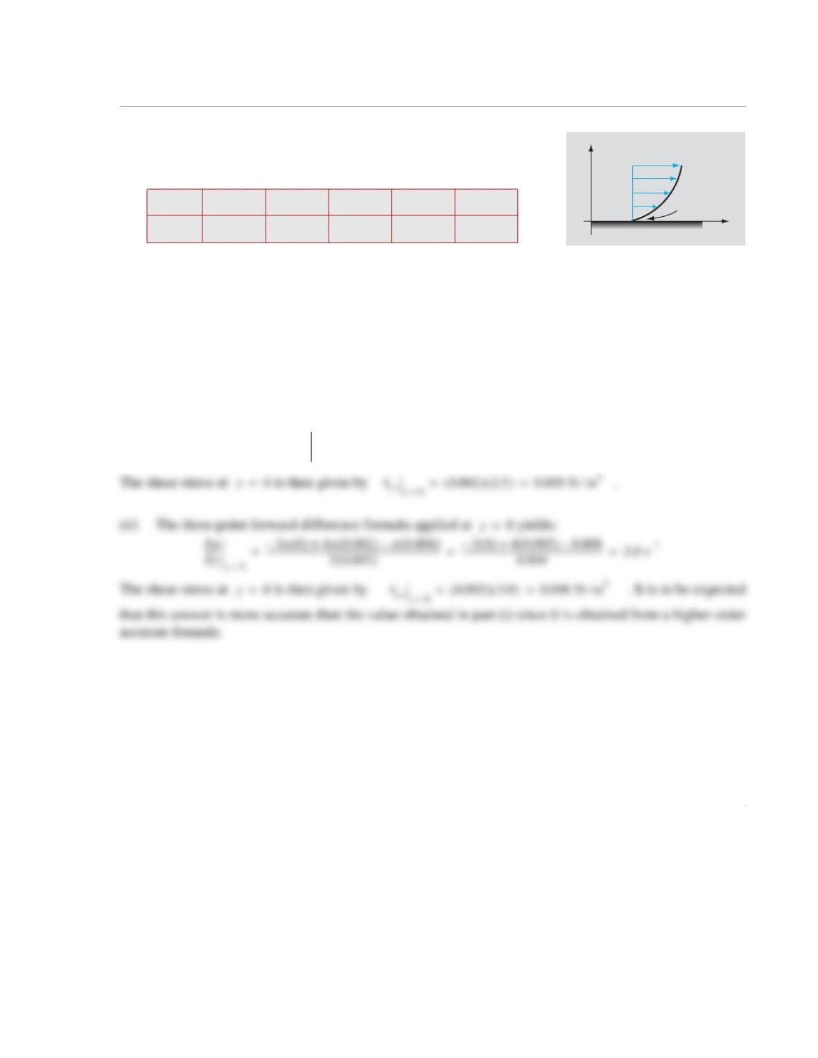
8.28 The distribution of the x-component of the velocity u of a fluid
near a flat surface is measured as a function of the distance y from the
surface:
The shear stress in the fluid is described by Newton’s equation:
where is the coefficient of dynamic viscosity. The viscosity can be thought of as a measure of the inter-
nal friction within the fluid. Fluids that obey Newton’s constitutive equation are called Newtonian fluids.
Calculate the shear stress at using (i) the two-point forward, and (ii) the three-point forward approx-
imations for the derivative. Take N-s/m2.
Solution
(i) The two-point forward difference formula applied at yields:
(m) 00.002 0.004 0.006 0.008
(m/s) 00.005 0.008 0.017 0.022
x
y
u(y)
τxy
y
u
τyx
τyx µu∂
y∂
—––
=
µ
y0=
µ0.00516=
y0=
u∂
y∂
—––
y0=
u0.002()u0()–
0.002
——————-——————- 0.005 0–
0.002
—————-—–– 2.5 s 1–
===
1
8.29 The refractive index n (how much the speed of light is reduced) of fused silica at different wave-
lengths is displayed in the table.
Use the data to calculate the dispersion (spreading of light beam) defined by at each wavelength.
(a) Use the user-defined function FirstDerivUneq written in Problem 8.23.
(b) Use MATLAB’s built-in function diff.
Solution
The two parts are solved in the following script file:
clear, clc,
L=[0.2 0.25 0.3 0.36 0.45 0.6 1.0 1.6 2.2 3.37]*1E-6;
When the script is executed, the following results are displayed in the Command Window:
Part (a)
Disa =
(m) 0.2 0.25 0.3 0.36 0.45 0.6 1.0 1.6 2.2 3.37
n1.551 1.507 1.488 1.475 1.466 1.458 1.450 1.443 1.435 1.410
λ
λ
µ
dn
dλ
—––
1
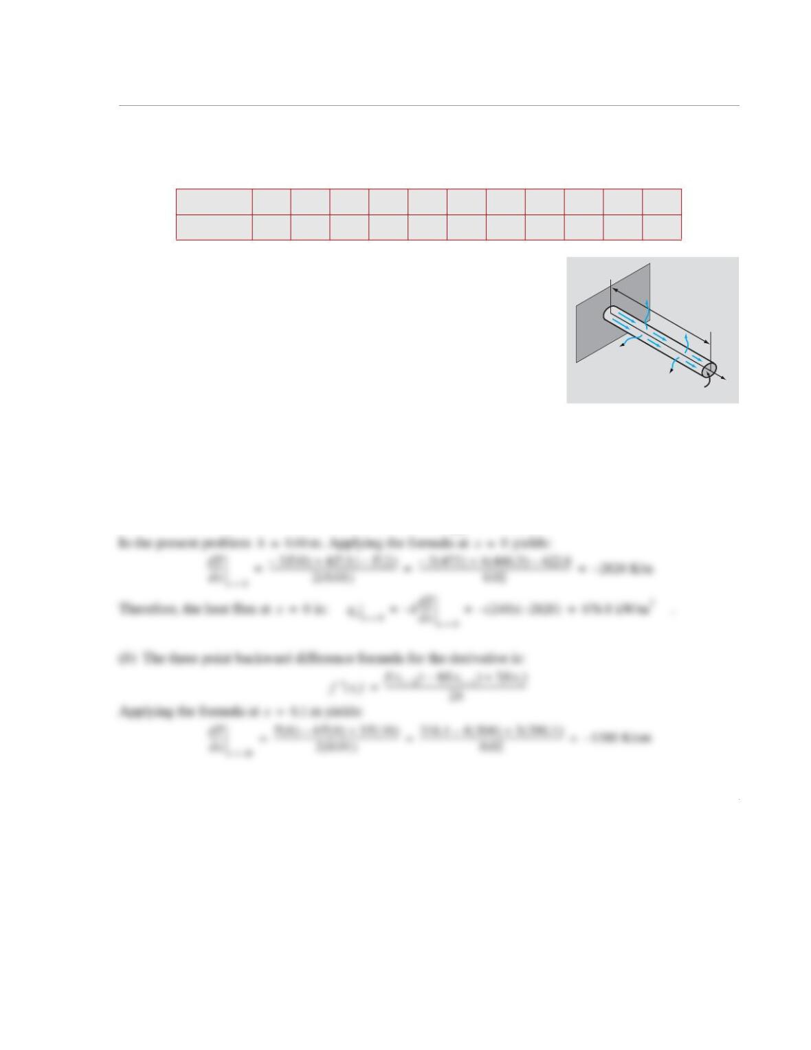
8.30 A fin is an extended surface used to transfer heat from a base material (at ) to an ambient. Heat
flows from the base material through the base of the fin, through its outer surface, and through the tip.
Measurement of the temperature distribution along a pin fin gives the following data:
The fin has a length cm, constant cross-sectional area of
m
2, and thermal conductivity W/m/K. The heat flux
(W/m2) is given by
(a) Determine the heat flux at . Use the three-point forward differ–
ence formula for calculating the derivative.
(b) Determine the heat flux at . Use the three-point backward dif-
ference formula for calculating the derivative.
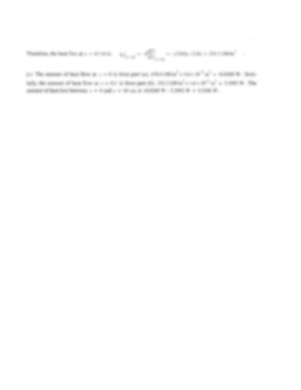
(c) Determine the amount of heat (in W) lost between and .
(The heat flow per unit time in Watts is the heat flux multiplied by the cross-sectional area of the fin.)
Solution
(a) The three point forward difference formula for the derivative is:
x (cm) 0 1 2 3 4 5 6 7 8 9 10
T (K) 473 446.3 422.6 401.2 382 364.3 348.0 332.7 318.1 304.0 290.1
x0=
TA
TB
TSx
L
L10=
1.6 10 5–
×
k240=
qxkdT
dx
—––
–=
x0=
xL=
x0=
xL=
f′xi
() 3fx
i
()–4fx
i1+
()fx
i2+
()–+
2h
——————-————————————————-–
=
x0=
x0=
2
1
8.31 The altitude of the space shuttle during the first two minutes of its ascent is displayed in the follow-
ing table (www.nasa.gov):
Assuming the shuttle is moving straight up, determine its velocity and acceleration at each point. Display
the results in three plots (h versus time, velocity versus time, and acceleration versus time).
(a) Solve by using the user-defined function FrstScndDerivPt that was written in Problem 8.19.
(b) Solve by using the MATLAB built-in function diff.
Solution
(a) The following scripts file uses the user-defined function FrstScndDerivPt that was written in
Problem 8.19 (b) to solve the problem. (The user-defined function FrstScndDerivPt was modified
such that the axes labels correspond to the variables in the current problem.)
t (s) 010 20 30 40 50 60 70 80 90 100 110 120
h (m) –8 241 1,244 2,872 5,377 8,130 11,617 15,380 19,872 25,608 31,412 38,309 44,726
2
(b) The following scripts file uses MATLAB built-in function diff to solve the problem.
020 40 60 80 100 120
-2
0
2
4
6x 10⁴
t (s)
h (m)
t (s)
3
clear, clc,
t=0:10:120;
h=[-8 241 1244 2872 5377 8130 11617 15380 19872 25608 31412 38309 44726];
dt=diff(t);
end
subplot(3,1,1)
plot(t,h); xlabel(‘t (s)’); ylabel(‘h (m)’);
subplot(3,1,2)
plot(tv,v); xlabel(‘t (s)’); ylabel(‘v (m/s)’);
subplot(3,1,3)
plot(ta,a); xlabel(‘t (s)’); ylabel(‘a (m/s^2)’);
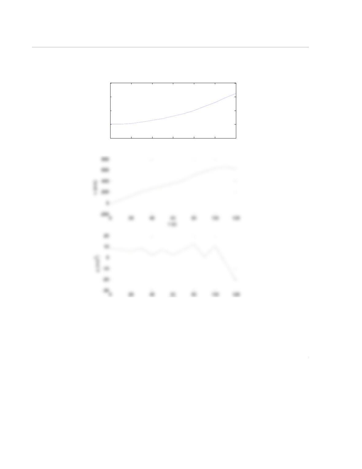
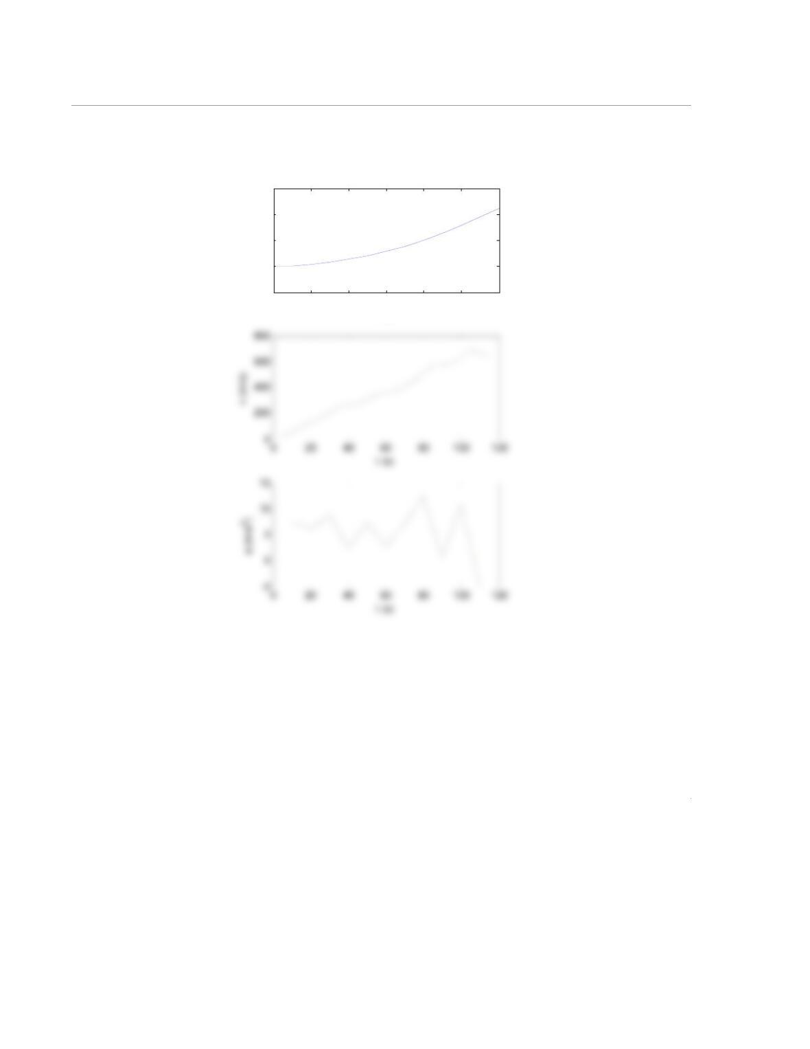
When the script is executed, the following results are displayed in the Command Window, and the follow-
ing figure is displayed.
4
020 40 60 80 100 120
-2
0
2
4
6x 10⁴
t (s)
h (m)
1
8.32 The position of an airplane at 5 s intervals as it accelerates on the runway is given in the following
table:
Write a MATLAB program in a script file that first determines the airplane’s velocity ( ) and the
acceleration ( ) at each point. Display the results in three plots (d versus time, velocity (in mph) ver-
sus time, and acceleration (in ft/s2) versus time).
(a) Solve by using the user-defined function FirstDeriv that was written in Problem 8.17.
(b) Solve by using the MATLAB built-in function diff.
Solution
(a) Script file:
t (s) 0 5 10 15 20 25 30 35 40
d (ft) 020 53 295 827 1437 2234 3300 4658
vdh
dt
—––
=
adv
dt
—––
=
2
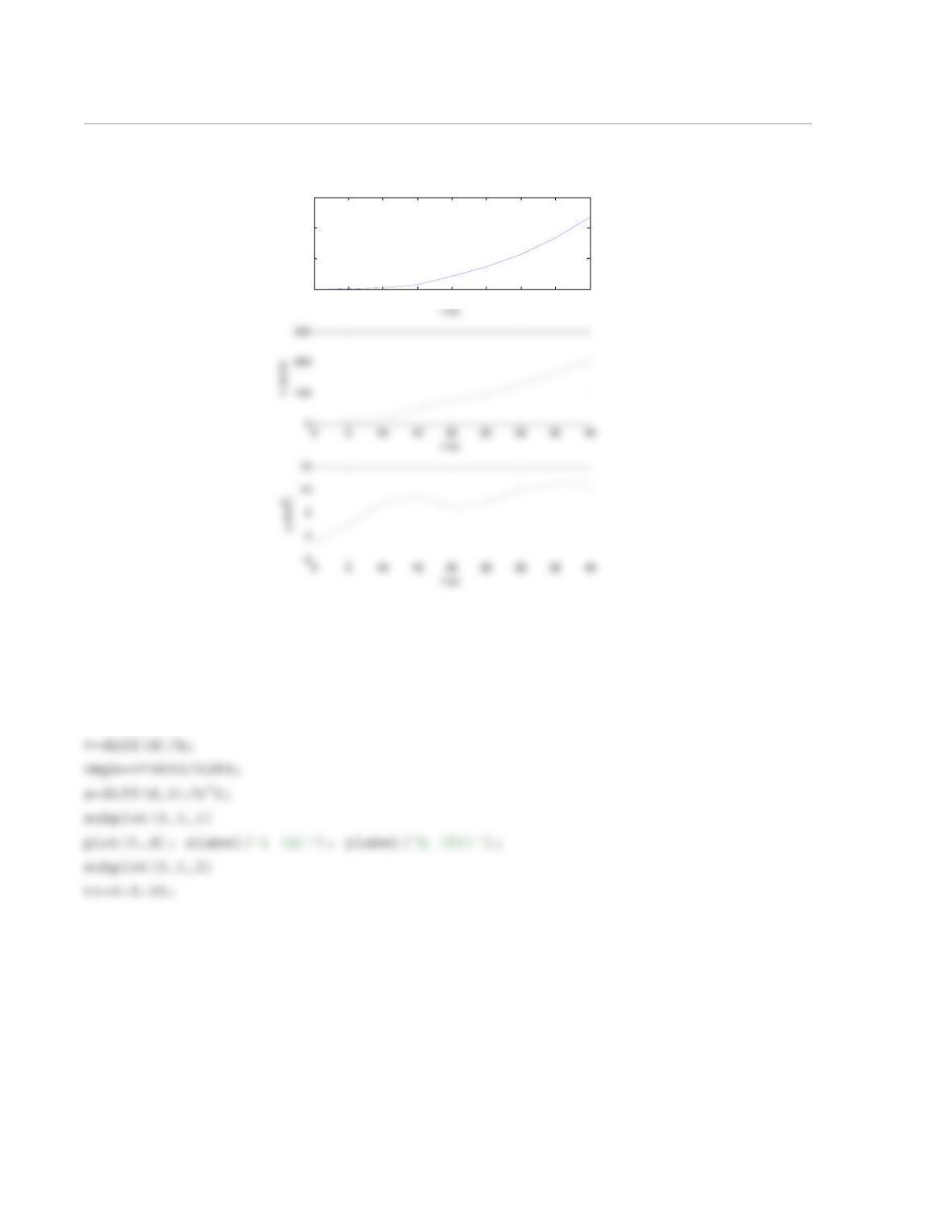
Figure Window:
(b) Script file:
t=0:5:40;
h=5;
d=[0 20 53 295 827 1437 2234 3300 4658];
0 5 10 15 20 25 30 35 40
0
2000
4000
6000
h (ft)
plot(tv,vmph); xlabel(‘t (s)’); ylabel(‘v (mi/h)’);
subplot(3,1,3)
ta=0:5:30;
plot(ta,a); xlabel(‘t (s)’); ylabel(‘a (ft/s^2)’);
Figure Window:
0 5 10 15 20 25 30 35 40
0
2000
4000
6000
t (s)
h (ft)
1
8.33 Use the user-defined function FrstScndDeriv written in Problem 8.19 to calculate the velocity
and the acceleration of the airplane in Problem 8.32. Display the results in three plots (h versus time, veloc-
ity versus time, and acceleration versus time).
Solution
Script file:
t=0:5:40;
d=[0 20 53 295 827 1437 2234 3300 4658];
[v,a] = FrstScndDeriv(t,d)
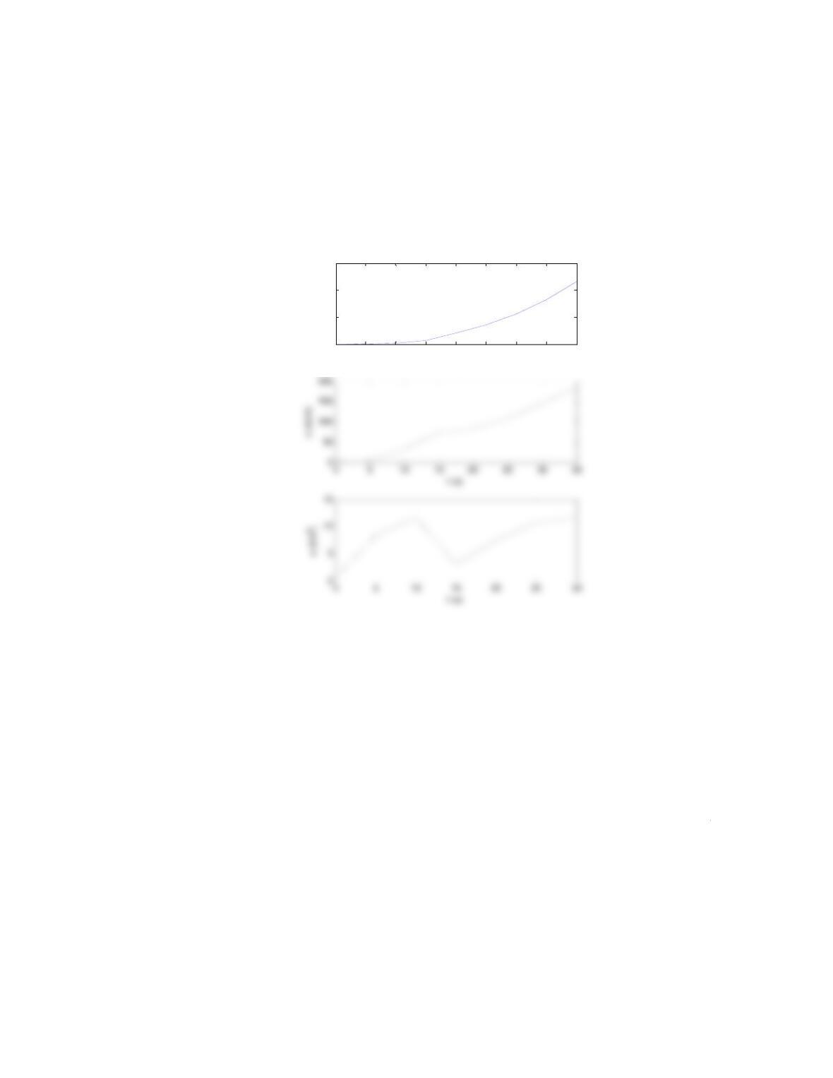
Figure Window:
0 5 10 15 20 25 30 35 40
0
2000
4000
6000
t (s)
h (ft)
1
8.34 The charge on the capacitor in the RC circuit shown at various
times after the switch is closed at time is given in the following
table. The current, I, as a function of time is given by .
Determine the current as a function of time by numerically differenti-
ating the data.
(a) Use the user-defined function FirstDerivUneq that was writ-
ten in Problem 8.23.
(b) Use the MATLAB built-in function diff.
In both parts plot I versus t.
Solution
(a) Script file:
(C) 0340 584 759 884 973 1038 1084 1117 1140 1157
t (ms) 050 100 150 200 250 300 350 400 450 500
(C) 1169 1178 1184 1189 1192 1194 1196 1197 1198 1199
t (ms) 550 600 650 700 750 800 850 900 950 1000
V0
R
+
_
I(t)
C
t0=
It() dQ
dt
——–
=
Q106
×
Q106
×
2
Figure:
(b) Script file:
Q=[0 340 584 759 884 973 1038 1084 1117 1140 1157 …
1169 1178 1184 1189 1192 1194 1196 1197 1198 1199]*1E-6;
t=[0:50:950]*0.001;
h=50*0.001;
6
7
8x 10⁻³