1
8.1 Given the following data:
find the first derivative at the point .
(a) Use the three-point forward difference formula.
(b) Use the three-point backward difference formula.
(c) Use the two-point central difference formula.
Solution
(a) The three point forward difference formula is given by (see Table 8-1):
1.1 1.2 1.3 1.4 1.5
0.6133 0.7822 0.9716 1.1814 1.4117
x
fx()
f′x()
x1.3=
f′xi
() 3fx
i
()–4fx
i1+
()fx
i2+
()–+
—————-———————————-——————–
=
1
8.2 Given the following data:
find the second derivative at the point .
(a) Use the three-point forward difference formula.
(b) Use the three-point backward difference formula.
(c) Use the three-point central difference formula.
Solution
(a) The three point forward difference formula is given by (see Table 8-1):
0.6 0.7 0.8 0.9 1.0
5.2296 3.6155 2.7531 2.2717 2
x
fx()
f′′ x()
x0.8=
f′xi
() 3fx
i
()–4fx
i1+
()fx
i2+
()–+
2h
—————-———————————-——————–
=
1
8.3 The following data show estimates of the population of Liberia in selected years between 1960 and
2010:
Calculate the rate of growth of the population in millions per year for 2010.
(a) Use two-point backward difference formula.
(b) Use three-point backward difference formula.
(c) Using the slope in 2010 from part (b), apply the two-point central difference formula to extrapolate and
predict the population in the year 2020.
Solution
(a) From Table 8-1, the two-point backward difference formula is:
Year 1960 1970 1980 1990 2000 2010
Population (millions) 1.1 1.4 1.9 2.1 2.8 4
f′xi
() fx
i
() fx
i1–
()–
h
—————–—————-–
=
1
8.4 The following data is given for the stopping distance of a car on a wet road versus the speed at which
it begins braking.
(a) Calculate the rate of change of the stopping distance at a speed of 62.5 mph using (i) the two-point
backward difference formula, and (ii) the three-point backward difference formula.
(b) Calculate an estimate for the stopping distance at 75 mph by using the results from part (a) for the
slope and the two-point central difference formula applied at the speed of 62.5 mph. How does the esti-
mate compares with the data?
Solution
(a) (i) The two-point backward difference formula for the rate of change of stopping distance with respect
to speed is given by (see Table 6-1):
v (mi/h) 12.5 25 37.5 50 62.5 75
d (ft) 20 59 118 197 299 420
1
8.5 Given three unequally spaced points , , and , use Taylor series expan-
sion to develop a finite difference formula to evaluate the first derivative / at the point . Verify
that when the spacing between these points is equal, the three-point forward difference formula is obtained.
The answer should involve , , and .
Solution
First write down the Taylor series expansions for and assuming the value is known:
xiyi
,()
xi1+ yi1+
,()
xi2+ yi2+
,()
dy
dx
xx
i
=
yi
yi1+
yi2+
yi1+
yi2+
yi
2
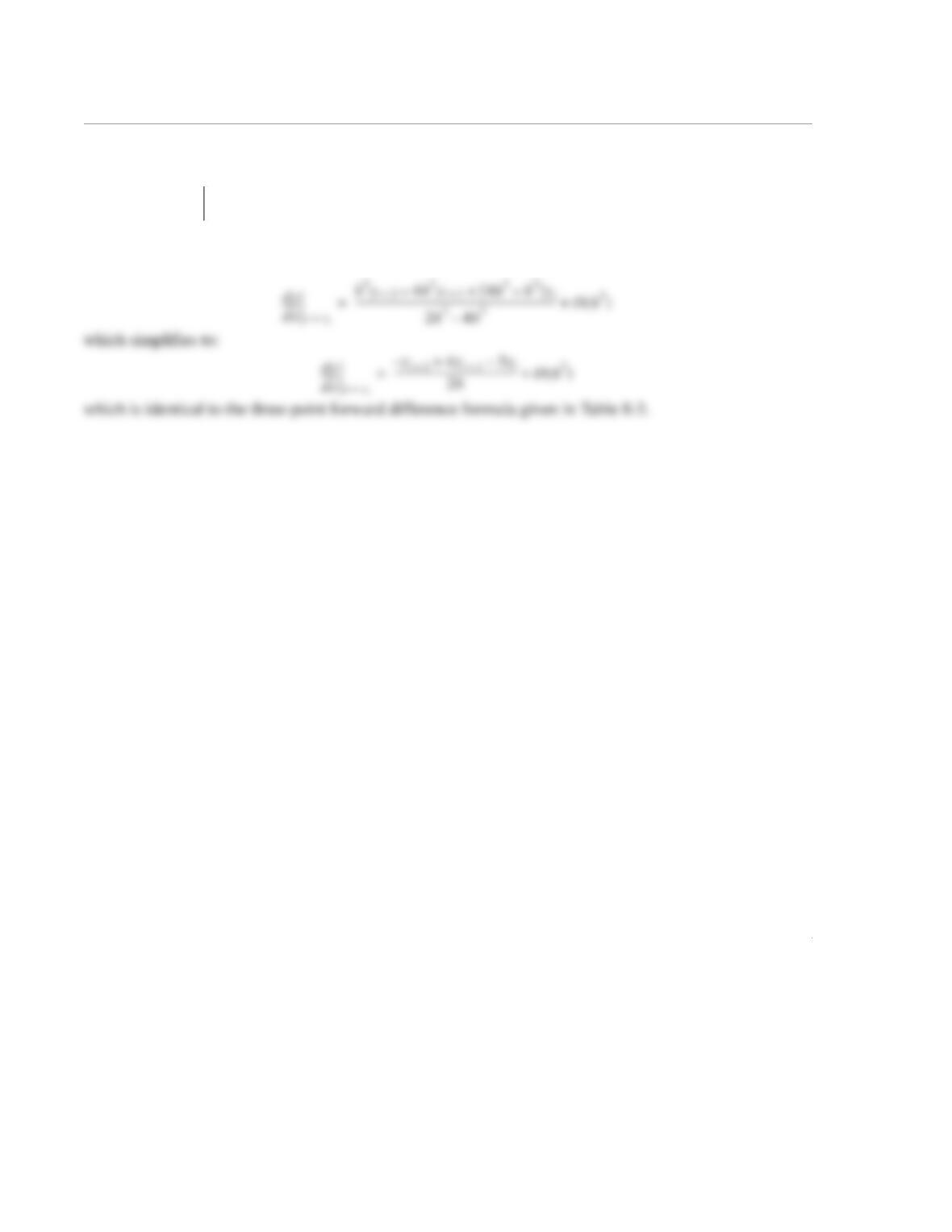
yields:
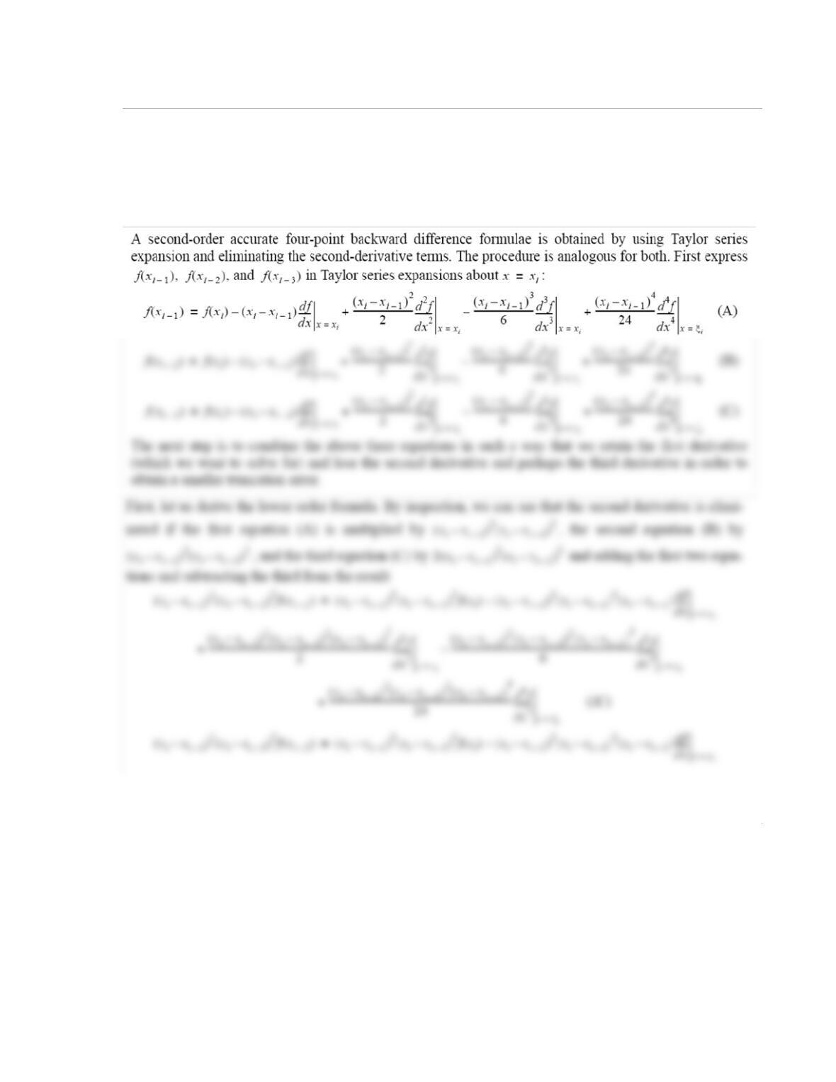
where TE is the truncation error. When the spacing between the points is equal, i.e.
and , the above expression reduces to:
dy
dx
—––
xx
i
=
xi1+ xi
–()
2yi2+ xi2+ xi
–()
2yi1+
–xi2+ xi
–()
2xi1+ xi
–()
2
–[]yi
+
xi1+ xi
–()
2xi2+ xi
–()xi2+ xi
–()
2xi1+ xi
–()–
—————————————————-———————————-———————————-———————————-——–TE+=
xi1+ xi
–xi2+ xi1+
–h==
xi2+ xi
–2h=
1
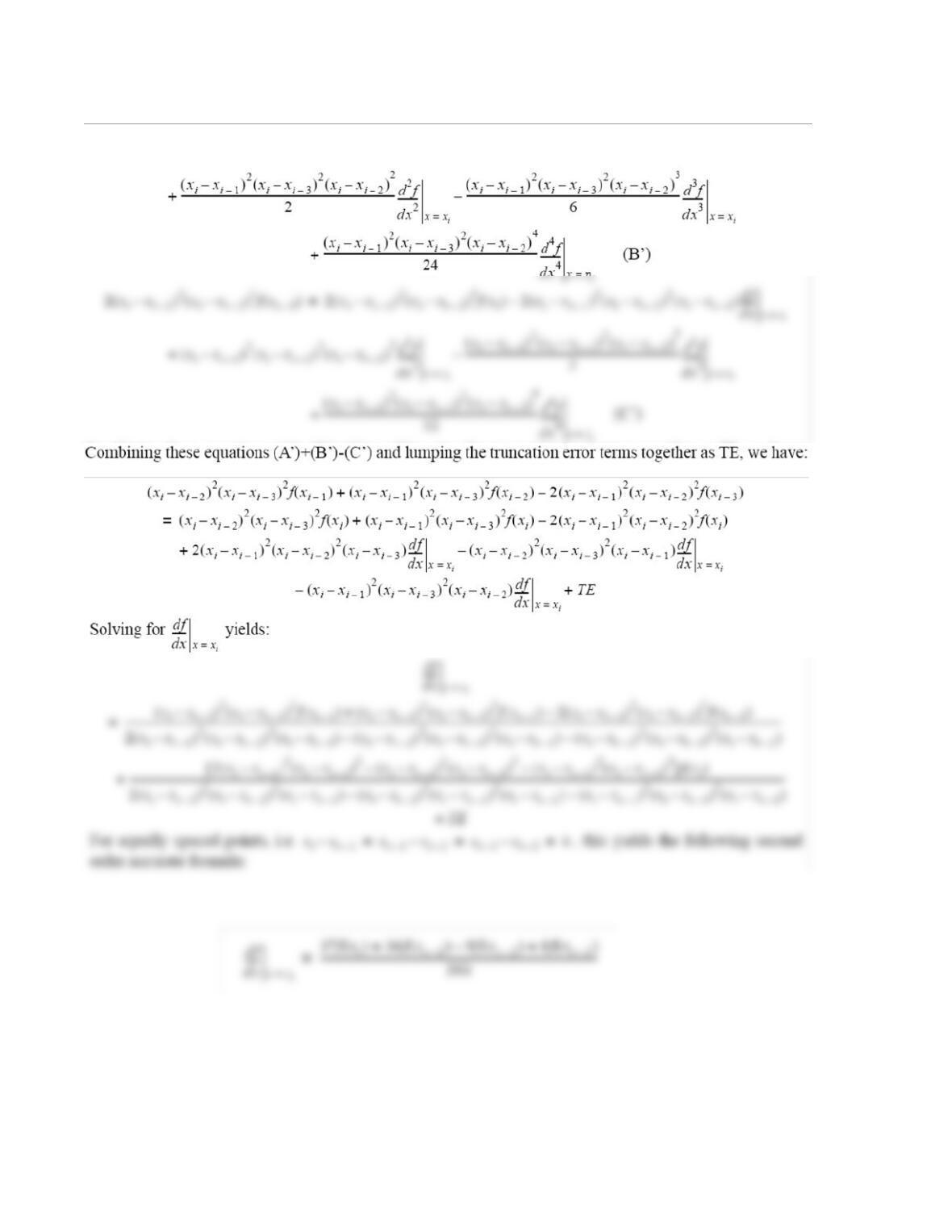
8.6 Using a four-term Taylor series expansion, derive a four-point backward difference formula for eval-
uating the first derivative of a function given by a set of unequally spaced points. The formula should give
the derivative at point , in terms of , , , , , , , and .
Solution
xx
i
=
xi
xi1–
xi2–
xi3–
fx
i
()
fx
i1–
()
fx
i2–
()
fx
i3–
()
2
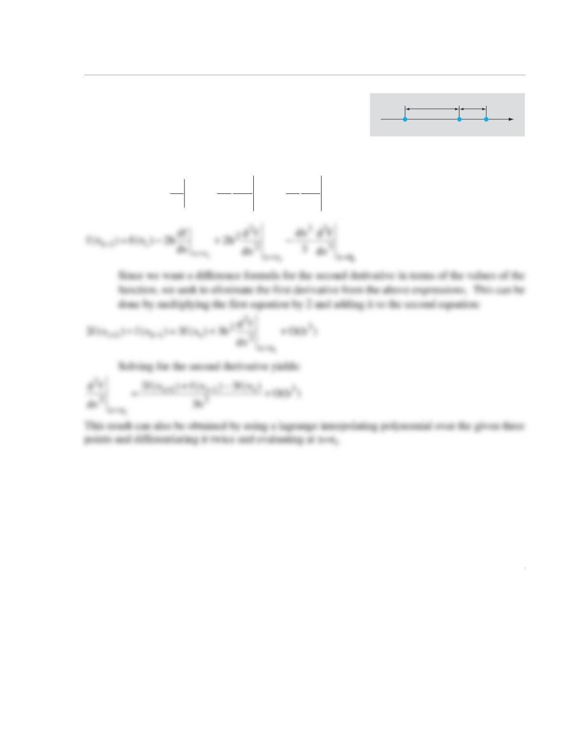
1
8.7 Derive a finite difference approximation formula for
using three points , , and , where the spacing is such that
and .
Solution
Expand f(xi+1) and f(xi-1) in terms of a Taylor series about x = xi:
x
xixi+1
xi–1
h
2h
f′′ xi
()
xi1–
xi
xi1+
xixi1–
–2h=
xi1+ xi
–h=
ii
ix
3
33
xx
2
22
xx
i1i dx
fd
6
h
dx
fd
2
h
dx
df
h)x(f)x(f
ξ==
=
++++=
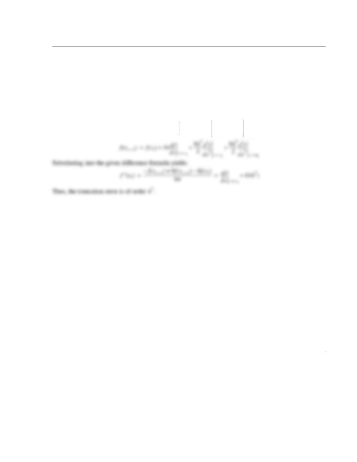
1
8.8 A particular finite difference formula for the first derivative of a function is:
where the points , , , and are all equally spaced with step size h. What is the order of the
truncation or discretization error?
Solution
The Taylor expansions are:
f′xi
() fx
i3+
()–9fx
i1+
()8fx
i
()–+
6h
—————–———————————-—————––
=
xi
xi1+
xi2+
xi3+
fx
i1+
()fx
i
() hdf
dx
—––
xx
i
=
h2
2
—-–d2f
dx2
——-–
xx
i
=
h3
6
—-–d3f
dx3
——-–
xξi
=
++ +=
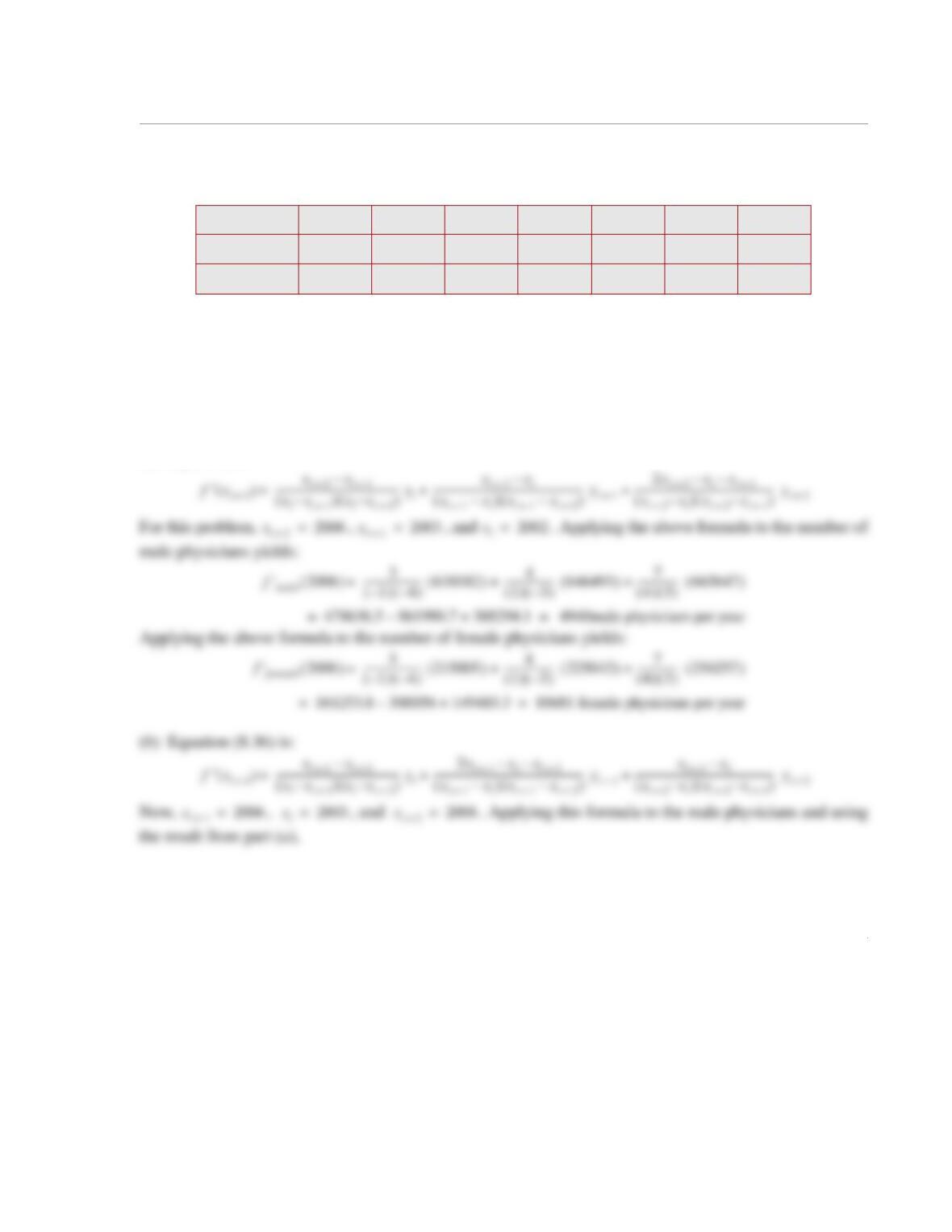
1
8.9 The following data show the number of female and male physicians in the U.S. for various years
(American Medical Association):
(a) Calculate the rate of change in the number of male and female physicians in 2006 by using the three-
point backward difference formula for the derivative, with unequally spaced points, Eq. (8.37).
(b) Use the result from part (a) and the three-point central difference formula for the derivative with
unequally spaced points, Eq. (8.36), to calculate (predict) the number of male and female physicians in
2008.
Solution
(a) Eq.(8.37) is:
Year 1980 1990 2000 2002 2003 2006 2008
# males 413,395 511,227 618,182 638,182 646,493 665,647 677,807
# females 54,284 104,194 195,537 215,005 225,042 256,257 276,417
2
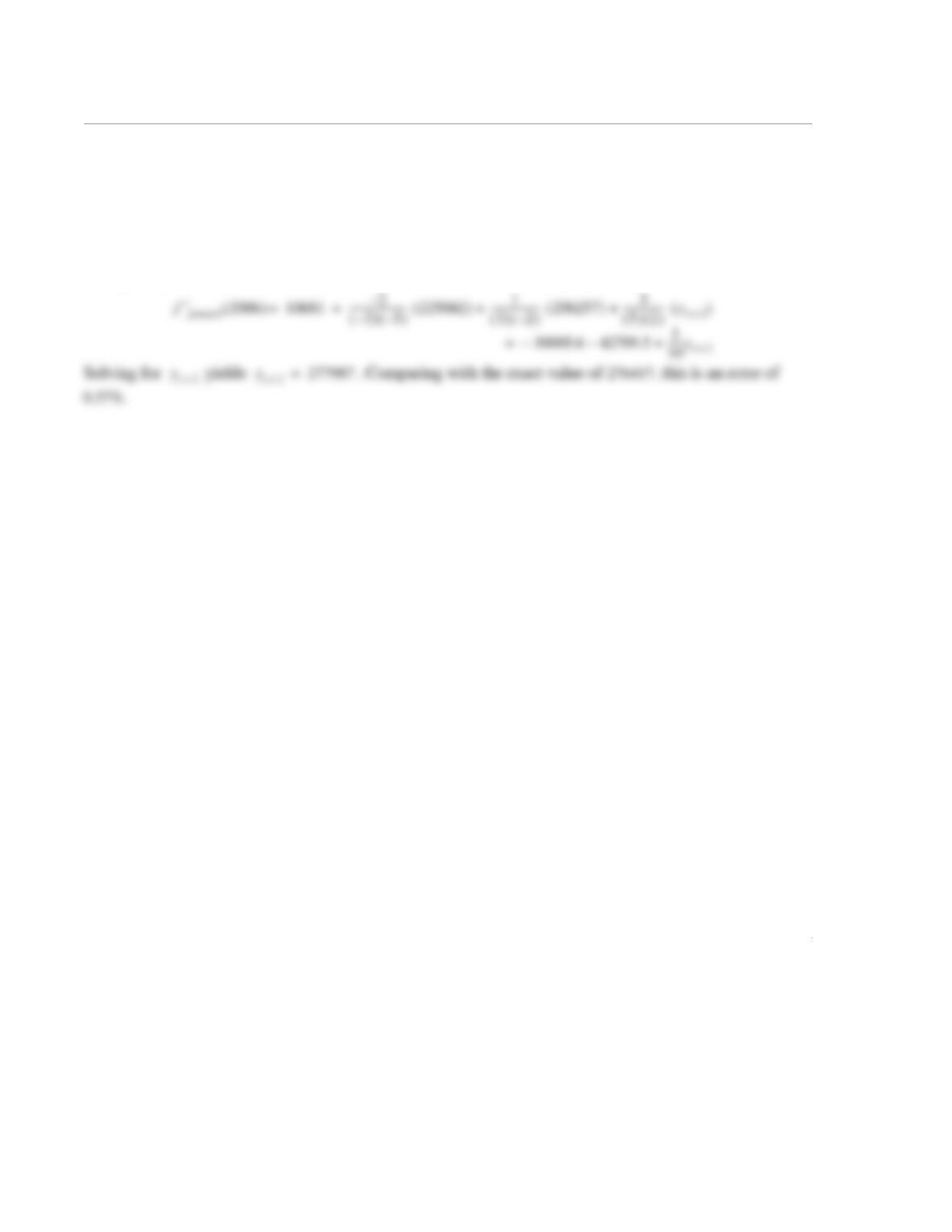
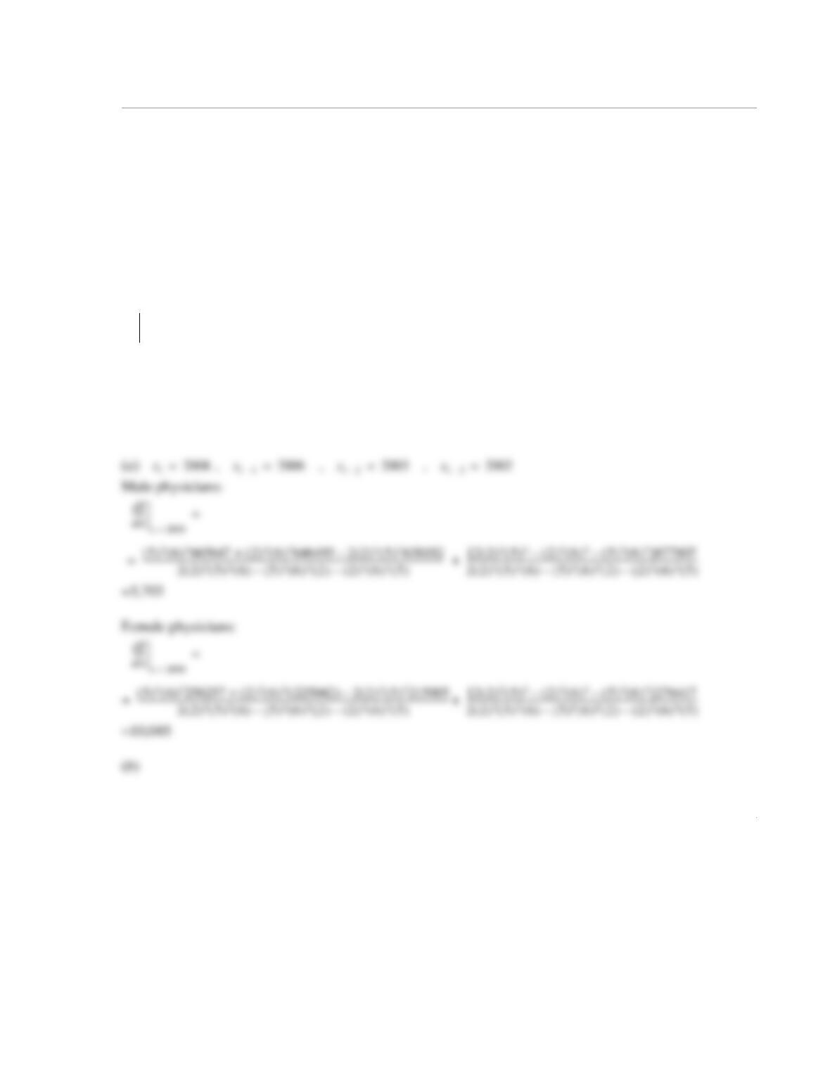
Solving for yields . Comparing with the exact value of 677807, this is in error by
0.62%. Applying the three-point ventral difference formula to the female physicians and using the result
from part (a),
f′male 2006()4940 2–
3–()5–()
—————–—-– 646493()
1
3() 2–()
——————–665647()
3
5()2()
—————–yi2+
()++
86199.1– 110941.2–3
10
—––yi2+
+
==
=
yi2+
yi2+ 673601=
1
8.10 Use the data from Problem 8.9 and the four-point backward difference formula that was derived in
Problem 8.6 for evaluating the first derivative of a function specified at unequally spaced points to calcu-
late the following quantities.
(a) Evaluate the rate of change in the number of male and female physicians in 2008.
(b) Use the data from 2008, 2006, together with the slopes in 2008 from part (a) to estimate the year in
which the number of female and male physicians will be equal. Use the three-point central difference
formula for the derivative (Eq. (8.36)) of a function specified at unequally spaced points.
Solution
The formula from Problem 8.6 is:
+
+
df
dx
—––
xx
i
=
=
xixi2–
–()
2xixi3–
–()
2fx
i1–
()xixi1–
–()
2xixi3–
–()
2fx
i2–
()2xixi1–
–()
2xixi2–
–()
2fx
i3–
()–+
2xixi1–
–()
2xixi2–
–()
2xixi3–
–()xixi2–
–()
2xixi3–
–()
2xixi1–
–()–xixi1–
–()
2xixi3–
–()
2xixi2–
–()–
—————————————————-———————————-———————————-———————————-———————————-———————————-———————————-—–
=
2xixi1–
–()
2xixi2–
–()
2xixi1–
–()
2xixi3–
–()
2
–xixi2–
–()
2xixi3–
–()
2
–[]fx
i
()
2xixi1–
–()
2xixi2–
–()
2xixi3–
–()xixi2–
–()
2xixi3–
–()
2xixi1–
–()–xixi1–
–()
2xixi3–
–()
2xixi2–
–()–
——————-———————————-———————————-———————————-—————————————————————-———————————–———————————-—-–
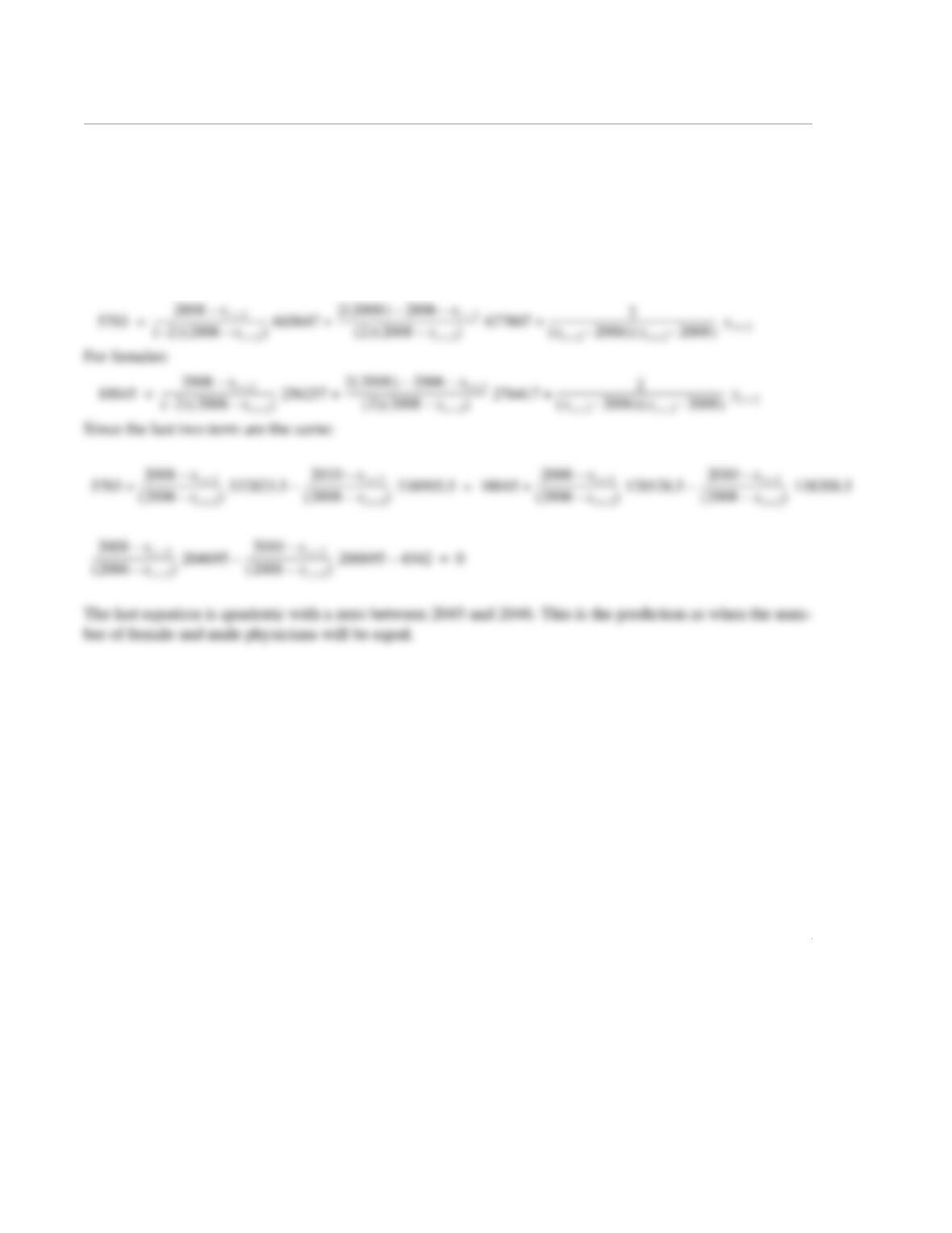
2
Equation (8.36):
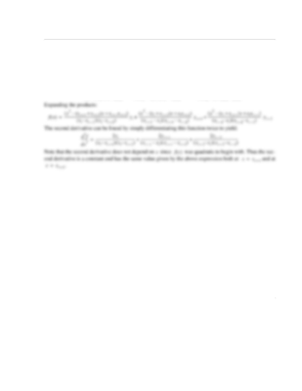
Use , and with to predict when is the same for male and
females.
For males:
f′xi1+
() xi1+ xi2+
–
xixi1+
–()xixi2+
–()
——————-—————————– yi
2xi1+ xi
–xi2+
–
xi1+ xi
–()xi1+ xi2+
–()
—————-———————————-——-–yi1+
xi1+ xi
–
xi2+ xi
–()xi2+ xi1+
–()
—————————————————-––yi2+
++=
xi2006=
xi1+ 2008=
f′2008()
xi2+
yi2+
1
8.11 Use Lagrange interpolation polynomials to find the finite difference formula for the second deriva-
tive at the point using the unequally spaced points , , and . What is the second deriva-
tive at and at ?
Solution
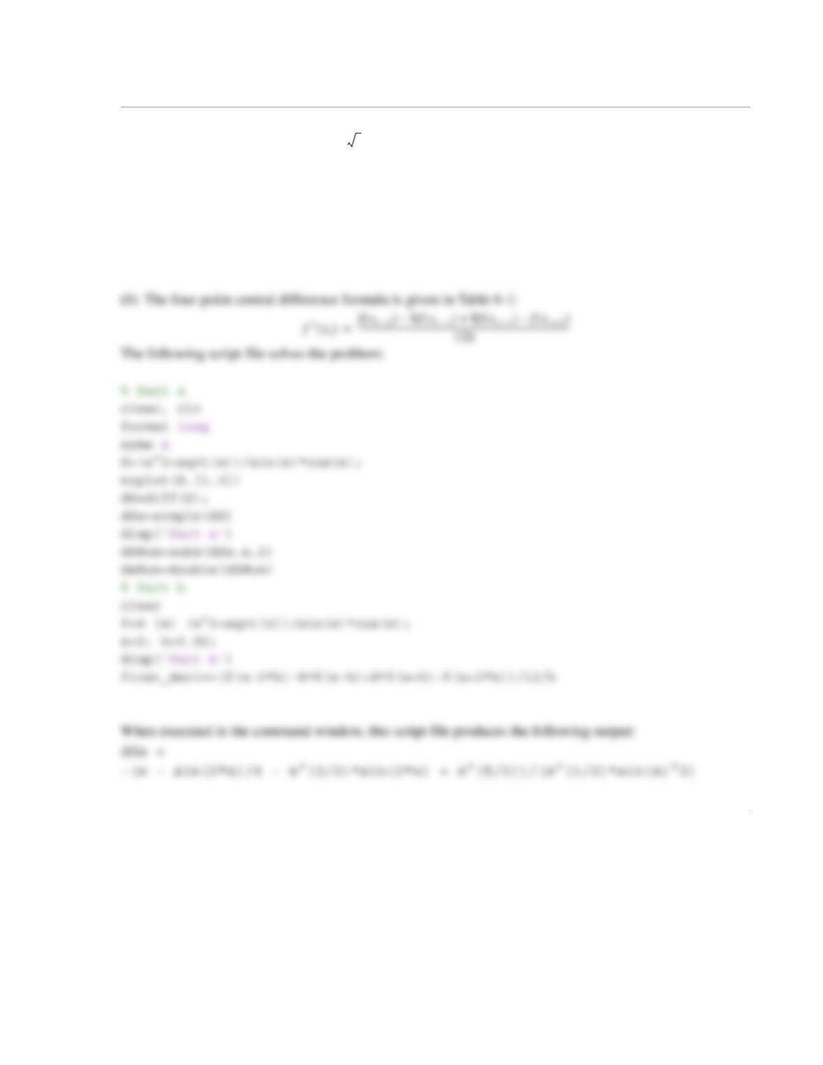
The Lagrange interpolation polynomial for these three points is given by Eq.(6.33) in Chapter 6:
xx
i
=
xi
xi1+
xi2+
xx
i1+
=
xx
i2+
=
fx() xx
i1+
–()xx
i2+
–()
xixi1+
–()xixi2+
–()
—————-——————————– yi
xx
i
–()xx
i2+
–()
xi1+ xi
–()xi1+ xi2+
–()
—————–———————————-——–yi1+
xx
i
–()xx
i1+
–()
xi2+ xi
–()xi2+ xi1+
–()
——————-———————————-–yi2+
++=
xx
=
1
8.12 Given the function , find the value of the first derivative at .
(a) Use analytical differentiation by hand.
(b) Use the four-point central difference formula with , , , and
. Write a MATLAB program in a script file to carry out the calculations.
Solution
(a) The derivative is found by using symbolic math in MATLAB
fx() x2x+()x()cos
x()sin
—————–———————-–
=
x2=
xi2– 1.96=
xi1– 1.98=
xi1+ 2.02=
xi2+ 2.04=
2
Part a
dSNum =
(2^(1/2)*(sin(4)/4 + 2*2^(1/2)*sin(4) – 4*2^(1/2) – 2))/(2*sin(2)^2)
1
8.13 For the function given in Problem 8.12, find the value of the second derivative at .
(a) Use analytical differentiation by hand.
(b) Use the five-point central difference formula with , , , ,
and . Write a MATLAB program in a script file to carry out the calculations.
Solution
(a) The derivative is found by using symbolic math in MATLAB
(b) The five-point central difference formula for the second derivative is given in Table 6-1:
The following script file calculates the derivative using this formula with :
% Part a
clear, clc
When executed in the command window, this script file produces the following output:
ddSs =
x2=
xi2– 1.96=
xi1– 1.98=
xi2=
xi1+ 2.02=
xi2+ 2.04=
f′′ xi
() fx
i2–
()–16fx
i1–
()30fx
i
()–16fx
i1+
()fx
i2+
()–++
12h2
—————————————————-———————————-—————-————————-–
=
h0.02=
2
(16*x^(5/2)*cos(x) + 8*x^2*sin(x) + 8*x^(7/2)*sin(x) – cos(x)^2*sin(x)
+ 4*x*cos(x) + 8*x^(3/2)*cos(x)^2*sin(x))/(4*x^(3/2)*cos(x)^3)
Part a
1
8.14 The following data for the velocity component in the x-direction, u, are obtained as a function of the
two coordinates x and y:
Use the four-point central difference formula for to evaluate this derivative at the point .
Solution
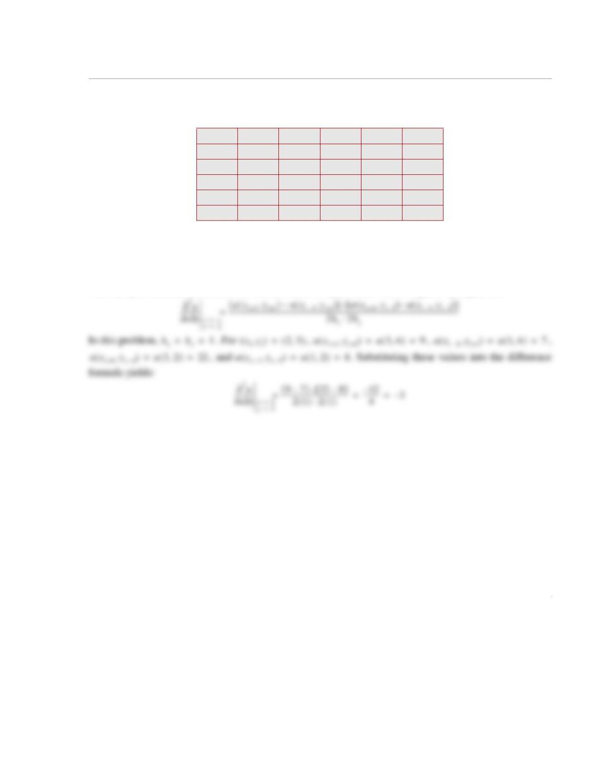
The four-point central difference formula for the mixed partial derivative is given by Eq.(6.65):
0 8 2 13 15
310 715 18
14 14 822 22
712 916 17
510 7 9 14
x0=
x1=
x2=
x3=
x4=
y0=
y1=
y2=
y3=
y4=
∂2u
∂y∂x
———––
23,()