3
function res = bcfunHW11_27b(ya,yb)
Tinf=300; h=100; k=72;
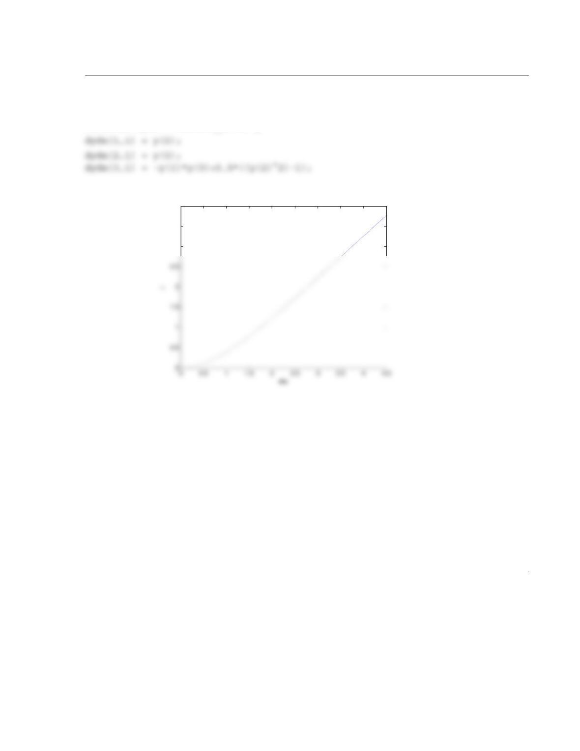
When executed, the program produces the following plot:
624.106
624.108
624.11
1
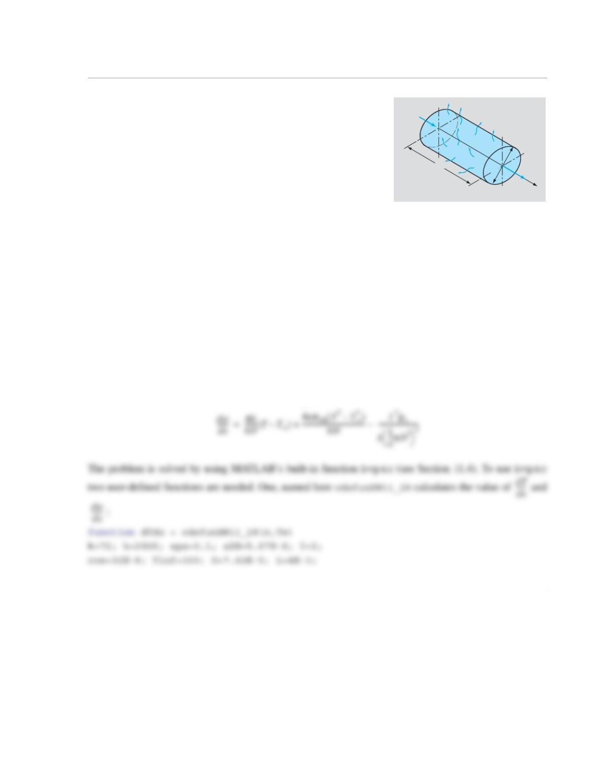
11.28 The axial temperature variation of a current-carrying bare wire
is described by:
where T is the temperature in K, x is the coordinate along the wire,
W/m/K is the thermal conductivity, W/m2/K2 is
the convective heat coefficient, is the radiative emissivity,
W/m2/K4 is the Stefan-Boltzmann constant,
A is the current, Ωm is the electrical resistivity, K is the ambient tempera-
ture, m is the wire diameter, and is the length of the wire. The boundary
conditions are:
at K, and at
Use MATLAB’s built-in function bvp4c to solve the boundary value problem for , since the tem-
perature distribution is symmetric about . Plot the temperature distribution along the wire.
Solution
The ODE is transforming into a system of two first-order ODEs:
T
8
I
Dx
L
I
d2T
dx2
———–4h
kD
——–TT
∞
–()–4εσSB T4T∞
4
–()
kD
——————-——————–
–I2ρe
k1
4
—–πD2
2
————————–
–=
k72=
h2000=
ε0.1=
σSB 5.67 10 8–
×=
I2=
ρe32 10 8–
×=
T∞300=
D7.62 10 5–
×=
L4.0 10 3–
×=
x0=
T300=
xL
2
—–
=
dT
dx
—–– 0=
0xL
2
—–
≤≤
xL
2
—–
=
dT
dx
—–– w=
2
dTdx = [Tw(2)
4*h*(Tw(1)-Tinf)/(k*D)+4*eps*sSB*(Tw(1)^4-Tinf^4)/(k*D)-I^2*roe/
(k*(pi*D^2/4)^2)];
The second user-defined function, named bcfunHW11_28 that computes the residual in the boundary con-
ditions:
The program in the following script file solves the problem:
% Solution HW11_28 (Script file)
clear
L=4E-3;
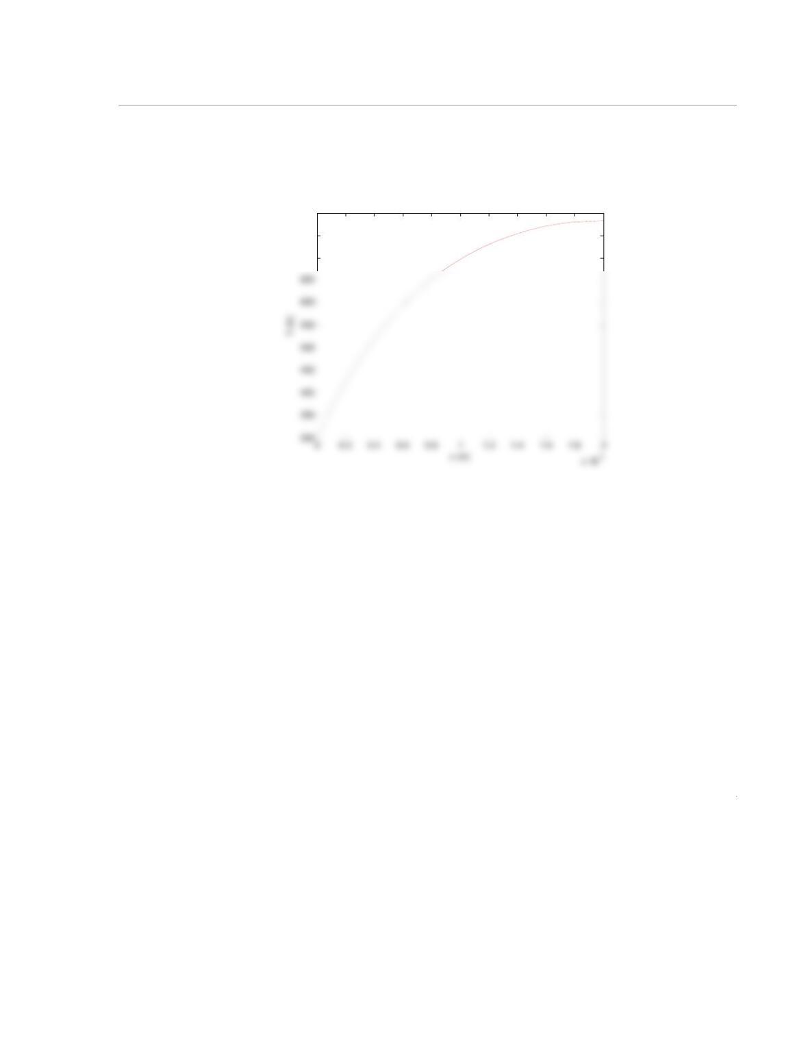
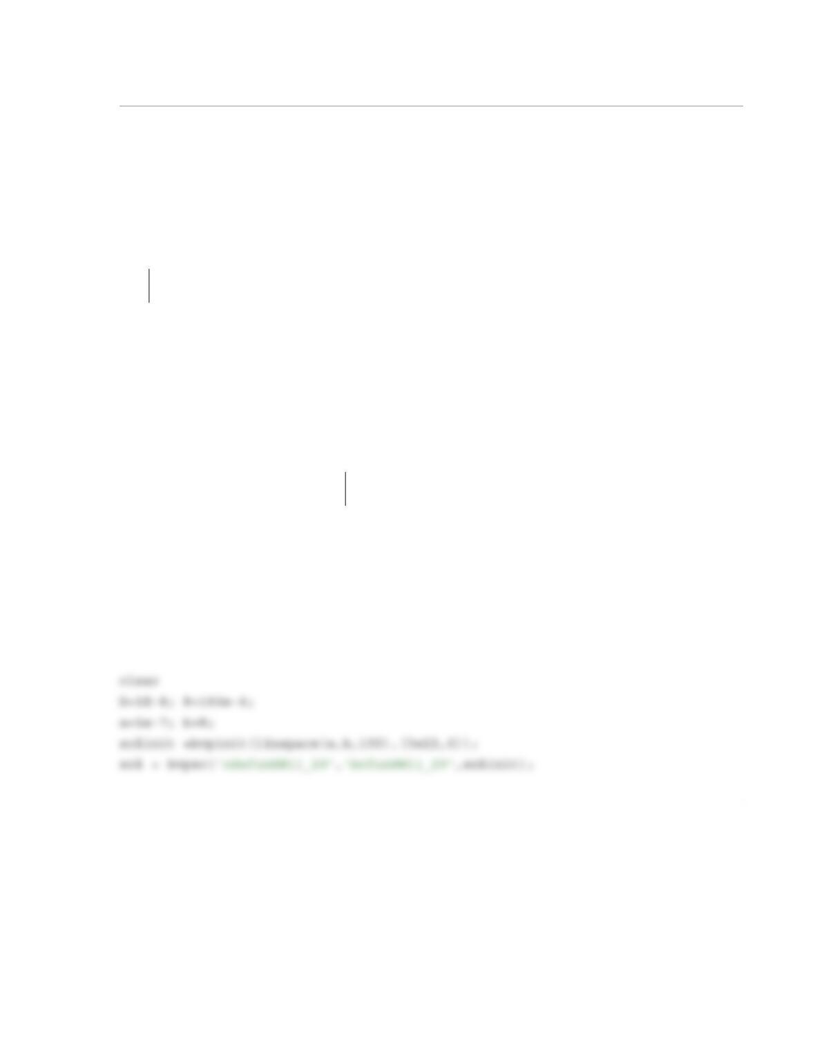
When the script file is executed, the following numerical solution is displayed in the Command Window,
and the following plot of the solution is displayed in the Figure Window:
Solution =
Columns 1 through 7
0 0.0001 0.0002 0.0003 0.0004 0.0005 0.0006
3
Columns 15 through 20
0.0015 0.0016 0.0017 0.0018 0.0019 0.0020
759.9591 767.9169 773.9759 778.2347 780.7626 781.6007
700
750
800
1
11.29 A spherical organism whose radius is m consumes O2 at a rate of s–1 throughout
its volume. The oxygen concentration at the surface of the organism is m–3, and its value in the
interior of the organism is governed by the following one-dimensional diffusion equation:
where m2/s is the diffusivity of O2. By symmetry, the boundary condition at is
.
(a) Rewrite the ODE as a system of two first-order ODEs and write down the boundary conditions.
(b) Solve the system of first-order ODEs using the MATLAB built-in function bvp4c for the steady state
distribution . Note that appears as a singularity on the right-hand side of one of the equa-
tions in part (a), and must therefore be replaced with a small (compared to R), non-zero value, e.g.,
m. Solve the equations from m to by dividing the domain into 100 subintervals,
and using initial guesses of and . Make a plot of versus r.
(c) Find the total rate of consumption of O2 by the organism, which is equal to the rate of diffusion of O2
at the surface, i.e., .
Solution
(a) Let . Then with the boundary conditions and
m-3.
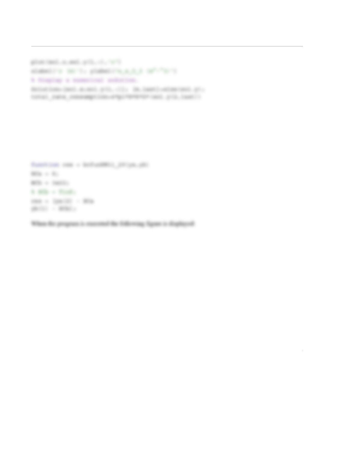
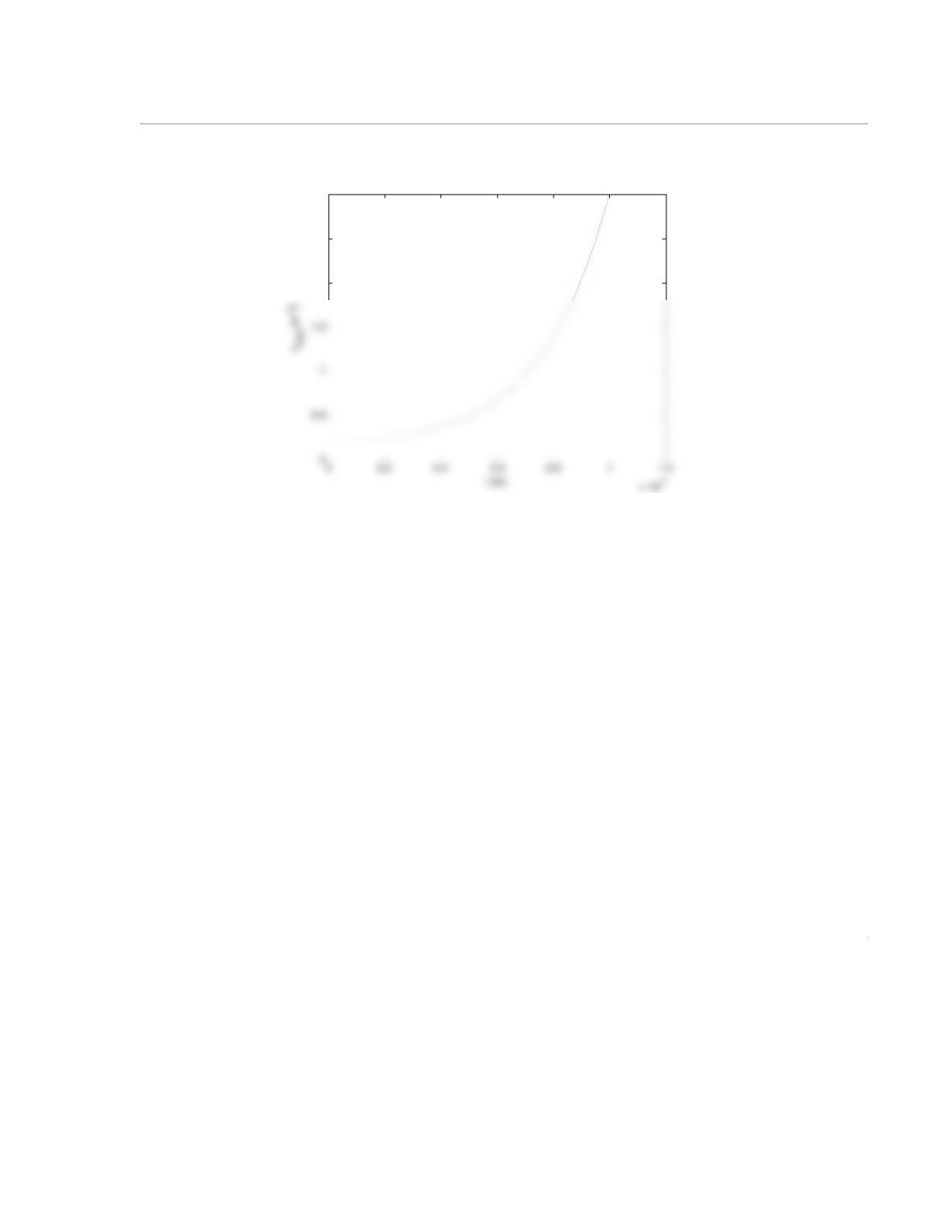
(b) The following script solves this problem:
R100=
µ
kO225=
310
22
×
1
r2
—– d
dr
—-– Dr2dnO2
dr
———-–
kO2nO2
–0=
D10 8–
=
r0=
dnO2
dr
———-–
r0=
0=
nO2r()
r0=
10 7–
r10 7–
=
rR=
nO2310
22
×=
dnO2
dr
———-–0=
nO2
RO24πrR2D
dnO2
dr
———-–
rR=
=
dnO2
dw
———-–w=
dw
dr
——–kO2nO2
D
————–– 2w
r
——–
–=
dnO2
dr
———-–0=
nO2rR=()310
22
×=
2
User-defined functions:
function dnO2dr = odefunHW11_29(r,nO2)
D=1e-8; kO2=25;
dnO2dr = [nO2(2)
(kO2*nO2(1)/D)-(2*nO2(2)/r)];
3
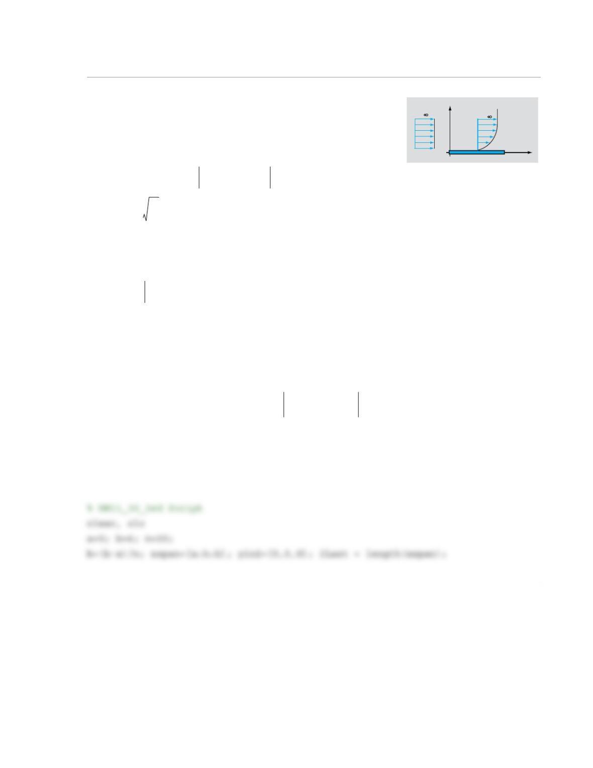
(c) On the command window, the following output is produced:
total_rate_consumption =
1.5081e+12
>>
2
2.5
3x 10²²
1
11.30 The velocity distribution in laminar boundary layer flow over a
flat plate is described by the solution of an ODE of the dimensionless
function (Blasius problem):
with the boundary conditions:
, , and
where is a dimensionless variable, and . The velocity components in the x and y direc-
tions are u and v, respectively. Solve this two-point boundary value problem for by rewriting the
third-order ODE as a system of three first-order ODEs. Solve the system as though it was an initial value
problem. This requires an assumed value for at that gives a solution that satisfies the boundary
condition . For the infinity boundary condition use . Write a MATLAB program in a
script file that uses MATLAB’s built-in functions to solve the system of the three ODEs. The program first
determines two values for that, when used in the solution, bound the boundary condition at infinity.
Then, the program uses the shooting method with linear interpolation (Eq. (11.14)) to determine the solu-
tion to the problem. To determine two values for that, when used in the solution bound the boundary
condition at infinity, start with the guess and , then use and , and so on.
Display the results in a plot of f versus , and a plot of versus (two separate figures).
Solution
The following script solves this problem:
x
y
uu
u
fη()
d3f
dη3
——––0.5 fd2f
dη2
——––
+0=
f0() 0=
df
dη
——
η0=
0=
df
dη
——
η∞→
1=
ηyu∞
vx
—––=
u
u∞
—––df
dη
——
=
fη()
d2f
dη2
——––
η0=
df
dη
——
η∞→
1=
η6=
d2f
dη2
——––
d2f
dη2
——––
d2f
dη2
——––
η0=
0=
d2f
dη2
——––
η0=
1
30
—––
=
1
30
—––
2
30
—––
η
df
dη
——
η
2
Yb=1;
% WL is the guessed value of the second derivative at x=a corresponding to
% the value YL of the first derivative calculated at x=b.
[x y] = ode45(@ODEHW11_30,xspan,yini); YL=y(iLast,2); WL=y(1,3);
User-defined function:
function dydx = ODEHW11_30(x, y)
dydx(1,1) = y(2);
dydx(2,1) = y(3);
dydx(3,1) = -0.5*y(1)*dydx(2,1);
3
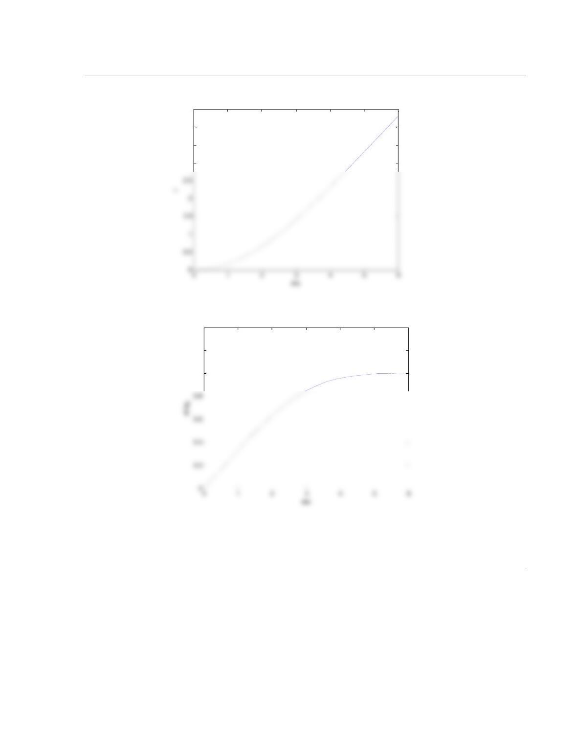
Executing this script results in the following plots:
3
3.5
4
4.5
1
1.2
1.4
1
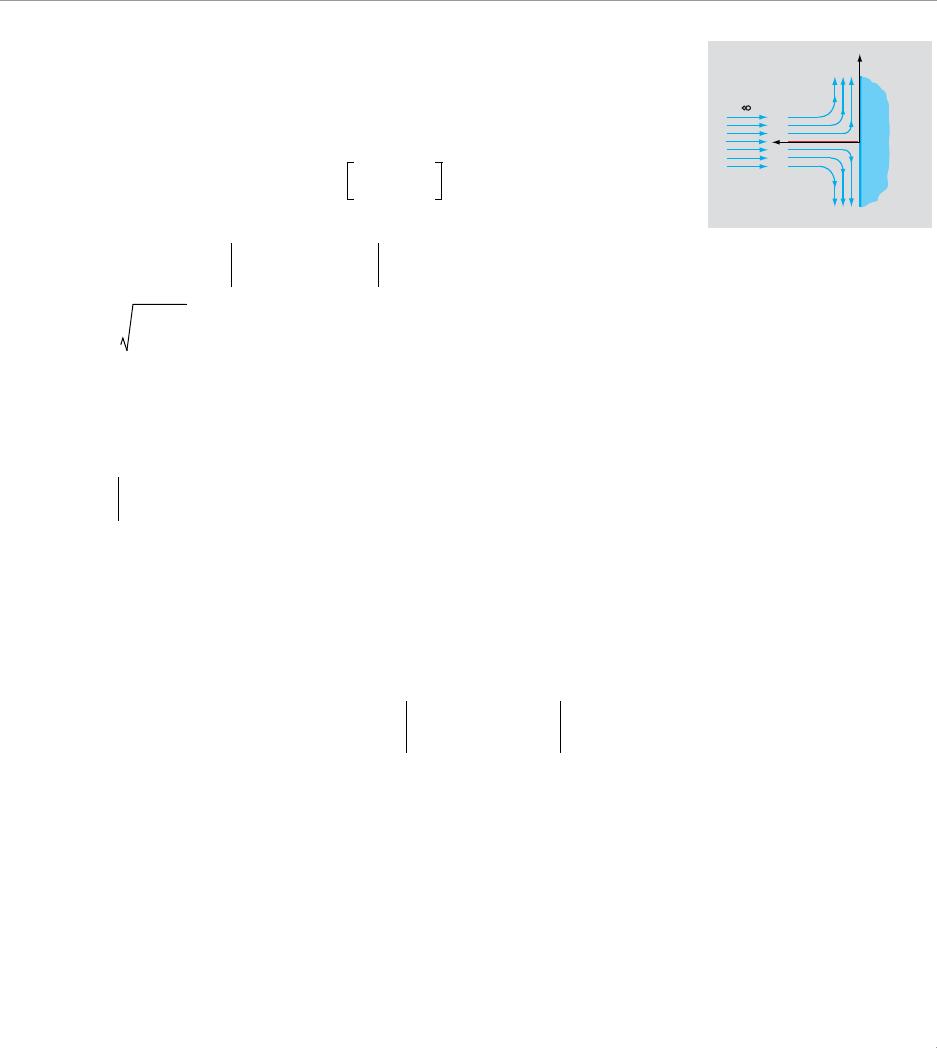
11.31 Stagnation plane flow of a fluid is encountered in welding applications.
For two-dimensional flow where the free stream horizontal component of
velocity is given by , the velocity distribution is determined by the
solution of the ODE for the non-dimensional function f :
with the boundary conditions:
, , and
where is dimensionless variable, and . The velocity components in the x and y
directions are u and v, respectively. Solve this two-point boundary value problem for by rewriting the
third-order ODE as a system of three first-order ODEs. Solve the system as though it was an initial value
problem. This requires an assumed value for at that gives a solution that satisfies the boundary
condition . For the infinity boundary condition use . Write a MATLAB program in a
script file that uses MATLAB’s built-in functions to solve the system of the three ODEs. The program first
determines two values for that, when used in the solution, bound the boundary condition at infinity.
Then, the program uses the shooting method with linear interpolation (Eq. (11.14)) to determine the solu-
tion to the problem. To determine two values for that, when used in the solution, bound the boundary
condition at infinity, start with the guess and , then use and , and so on.
Display the results in a plot of f versus , and a plot of versus (two separate figures). Note that
replacing with a number greater than 4.5 will cause numerical problems as the second derivative
vanishes and changes the ODE.
Solution
The following script solves this problem:
x
y
u
u∞Cx13⁄
=
d3f
dη3
——––fd2f
dη2
——––0.5 df
dη
——
2
1––+0=
f0() 0=
df
dη
——
η0=
0=
df
dη
——
η∞→
1=
ηy2C
3vx23⁄
—————–=
u
u∞
—––df
dη
——
=
fη()
d2f
dη2
——––
η0=
df
dη
——
η∞→
1=
η4.5=
d2f
dη2
——––
d2f
dη2
——––
d2f
dη2
——––
η0=
0=
d2f
dη2
——––
η0=
1
30
—––
=
1
30
—––
2
30
—––
η
df
dη
——
η
η∞→
d2f
dη2
——––
2
% HW11_31_3ed
clear
% Checking if Yb is between the two solutions.
if (Yb > YL & Yb < YH) | (Yb > YH & Yb < YL)
% Use Eq.(11.14):
WN=WL+((Yb-YL)*(WH-WL)/(YH-YL));
[x y] = ode45(@ODEHW11_31,xspan,yini);
figure(1)
plot(x,y(:,1));
3
User-defined function:
function dydx = ODEHW11_31(x, y)
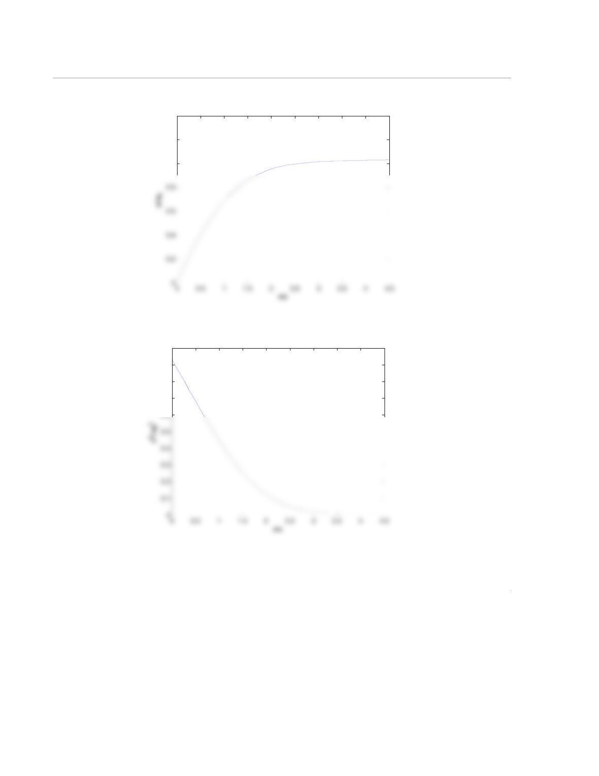
Executing this script results in the following plots:
3
3.5
4
4
1
1.2
1.4
0.7
0.8
0.9
1