Chapter 9 Homework Determine The Volume The Silo Problem

1

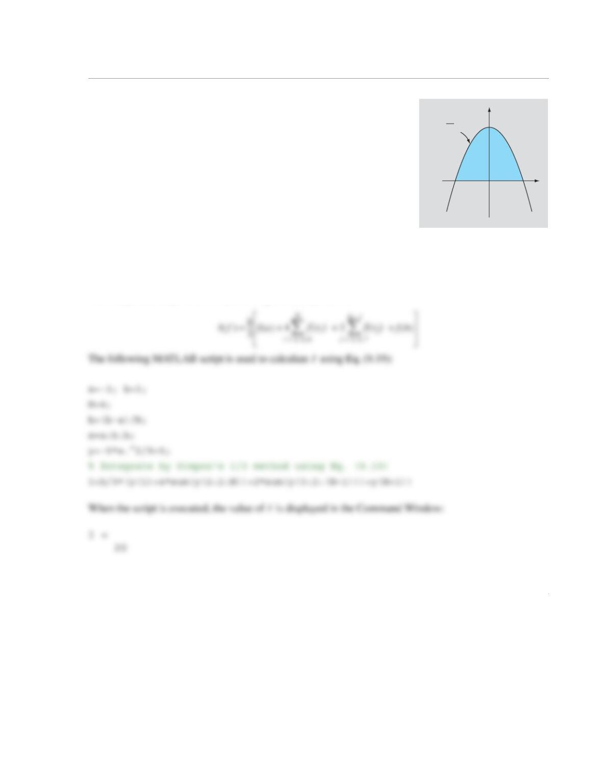
9.9 The area of the shaded region shown in the figure can be calculated

by:

Evaluate the integral using the following methods:

(a) Simpson’s 1/3 method. Divide the whole interval into four

subintervals.

(b) Simpson’s 3/8 method. Divide the whole interval into nine

subintervals.

(c) Three-point Gauss quadrature.

Compare the results and discuss the reasons for the differences.

Solution

(a) For , .

The composite Simpson’s 1/3 method is given by Eq. (9.19):

x

y

5

3

-3

y = – x

2

+ 5

5

9

A5

9

—–x2

–5+





xd

3–

3

20==

N4=

hba–

N

———––1.5==

2

(b) For , . Eq. (9.22) is used to calculate the integral using Simpson’s 3/8

method:

The following MATLAB script is used to calculate using Eq. (7.22):

When the script is executed, the value of is displayed in the Command Window:

I =

20

N9=

hba–

N

———––2

3

—–

==

If() 3h

8

—––fa() 3fx

i

() fx

i1+

()+[]

i258,,=

N1–

2fx

j

()

j4710,,=

N2–

fb()+++≈

I

3

where , , , , , and

. The calculations are done in the following script file:

When the script is executed, the following answer isplayed in the Command Window:

I =

fx()xd

1–

1

C1fx

1

()C2fx

2

()C3fx

3

()++≈

C10.5555556=

x10.77459667–=

C20.8888889=

x20=

C30.5555556=

x30.77459667=

1

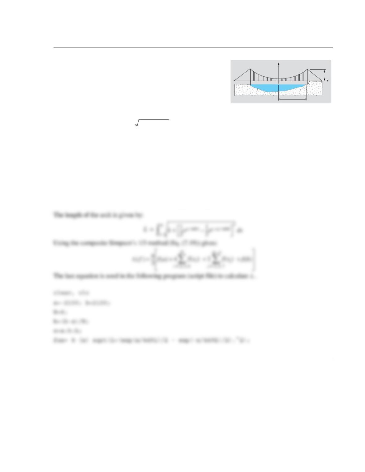
9.10 The central span of the Golden Gate bridge is 4200 ft long

and the towers’ height from the roadway is 500 ft. The shape of

the main suspension cables can be approximately modeled by the

equation:

for ft

where .

By using the equation , determine the length of the main suspension cables with

the following integration methods:

(a) Simpson’s 1/3 method. Divide the whole interval into eight subintervals.

(b) Simpson’s 3/8 method. Divide the whole interval into nine subintervals.

(c) Three-point Gauss quadrature.

Solution

(a) For ,and evenly-spaced points ft. The derivative of is:

x

y

2100 ft

500 ft

fx() CexC⁄exC⁄–

+

2

—————-————– 1–





=

2100– x2100≤≤

C4491=

L1f′x()[]

2

+xd

a

b



=

N8=

hba–

N

———––2 2100()

8

—————–—–525== =

fx()

f‘x() 1

2

—–ex4491⁄1

2

—–ex–()4491⁄

–=

2

When the script is executed, the value of is displayed in the Command Window:

L =

4.354742601750319e+03

The length of the arch as calculated by Simpson’s 1/3 method is ft.

The last equation is used in the following program (script file) to calculate .

clear, clc

a=-2100; b=2100;

When the script is executed, the value of is displayed in the Command Window:

L =

L

L4354.7=

L

3

4.354744421120988e+03

The length of the arch as calculated by Simpson’s 3/8 method is ft.

Three-point Gauss quadrature:

where , , , , , and

. The calculations are done in the following script file:

clear, clc

C1=0.5555556; C2=0.8888889; C3=0.5555556;

x1=-0.77459667; x2=0; x3=0.77459667;

L4354.7=

fx()xd

1–

1

C1fx

1

()C2fx

2

()C3fx

3

()++≈

C10.5555556=

x10.77459667–=

C20.8888889=

x20=

C30.5555556=

x30.77459667=

1

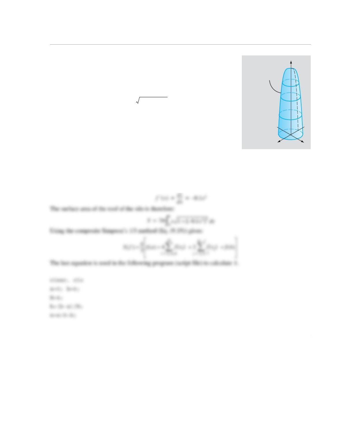
9.11 A silo structure is made by revolving the curve

from m to m about the z-axis, as shown in the figure to the

right.

The surface area, S, that is obtained by revolving a curve in

the domain from a to b around the z-axis can be calculated by:

Calculate the surface area of the silo with the following integration meth-

ods:

(a) Simpson’s 1/3 method. Divide the whole interval into four subinter–

vals.

(b) Simpson’s 3/8 method. Divide the whole interval into six subintervals.

(c) Three-point Gauss quadrature method.

Solution

(a) The limits of integration are and . For and evenly-spaced points

m. The derivative of is:

xy

32.4

z = – 0.025x4 + 32.4

6

z

z0.025x4

– 32.4+=

x0=

x6=

zfx()=

S2πx1f′x()[]

2

+xd

a

b



=

a0=

b6=

N4=

hba–

N

———––1.5==

fx()

2

fun= @ (x) x.*sqrt(1+(-0.1*x.^3).^2);

y=fun(x);

% Integrate by Simpon’s 1/3 method using Eq. (9.19)

S=h/3*(y(1)+4*sum(y(2:2:N))+2*sum(y(3:2:(N-1)))+y(N+1));

S=S*2*pi

When the script is executed, the value of is displayed in the Command Window:

The last equation is used in the following program (script file) to calculate .

clear, clc

a=0; b=6;

N=6;

h=(b-a)/N;

x=a:h:b;

S

3

When the script is executed, the value of is displayed in the Command Window:

S =

9.979516437653208e+02

The surface area of the silo roof as calculated by Simpson’s 3/8 method is m2.

(c) The coefficients and Gauss points for second-order Gauss quadrature are given in Table 9-1 and are

valid if the range of integration is . Because the range of integration in the present problem is ,

the integral must be rewritten according to Eq. (9.31):

Three-point Gauss quadrature:

where , , , , , and

. The calculations are done in the following script file:

clear, clc

When the script is executed, the value of is displayed in the Command Window:

S =

S

997.95

1–1,[]

06,[]

0

2π3t3+()10.13t3+()

1–



fx()xd

1–

1

C1fx

1

()C2fx

2

()C3fx

3

()++≈

C10.5555556=

x10.77459667–=

C20.8888889=

x20=

C30.5555556=

x30.77459667=

S

9.948814767300926e+02

994.88

1

9.12 Determine the volume of the silo in Problem 9.11. The volume, V, that is obtained by revolving a

curve in the domain from a to b around the z-axis can be calculated by:

Calculate the volume of the silo with the following integration methods:

(a) Simpson’s 1/3 method. Divide the whole interval into four subintervals.

(b) Simpson’s 3/8 method. Divide the whole interval into six subintervals.

(c) Three-point Gauss quadrature.

Solution

xfz()=

Vπfz()[]

2zd

a

b



=

z0.025x4

– 32.4+=

x40 z– 32.4+()[]

14⁄

=

Vπfz()[]

2zd

a

b

π40 z– 32.4+()[]

12⁄zd

a

b



==

2

y=fun(x);

% Integrate by Simpon’s 1/3 method using Eq. (9.19)

I=h/3*(y(1)+4*sum(y(2:2:N))+2*sum(y(3:2:(N-1)))+y(N+1));

V=I*pi

When the script is executed, the value of is displayed in the Command Window:

The last equation is used in the following program (script file) to calculate .

clear, clc

a=0; b=32.4;

When the script is executed, the value of is displayed in the Command Window:

V

3

V =

2.4183e+03

The volume of the silo as calculated by Simpson’s 3/8 method is m3.

Three-point Gauss quadrature:

where , , , , , and

. The calculations are done in the following script file:

clear, clc

2418.3

1–

fx()xd

1–

1

C1fx

1

()C2fx

2

()C3fx

3

()++≈

C10.5555556=

x10.77459667–=

C20.8888889=

x20=

C30.5555556=

x30.77459667=

The volume of the silo as calculated by the second-order Gauss quadrature method is m3.2452.1

1

9.13 In the standard Simpson’s 1/3 method (Eq. (9.16)), the points used for the integration are the

endpoints of the domain, a and b, and the middle point . Derive a new formula for Simpson’s 1/3

method in which the points used for the integration are , , and .

Solution

Starting with the polynomial given by Eq.(9.15),

or,

where . Substituting for yields:

ab+()2⁄

xa=

xb=

xab+()3⁄=

px() fx

1

() fx

2

()fx

1

()–[]

x2x1

–()

—————–—————–– xx

1

–() fx

3

()fx

1

()–

x3x1

–()x3x2

–()

—————-—————-———–fx

2

()fx

1

()–

x2x1

–()x3x2

–()

——————-———————-–

–xx

1

–()xx

2

–()++=

Ifa()ba–()

fx

2

()fa()–[]

2x2a–()

—————–————–– ba–()

2b

6

—–fb() fa()–

ba–()bx

2

–()

————————————–fx

2

()fa()–

x2a–()bx

2

–()

—————–——————––

–ba–()

2

++=

x2ab+()3⁄=

x2

1

9.14 The value of can be calculated from the integral .

(a) Approximate using the composite trapezoidal method with six subintervals.

(b) Approximate using the composite Simpson’s 1/3 method with six subintervals.

Solution

(a) The composite trapezoidal method is given by Eq. (9.13):

π

π1

2

—–4

1x2

+

————-–xd

1–

1



=

π

If() h

2

—–fa() fb()+

[]hfx

i

()

i2=

N



+≈

2

a=-1; b=1;

N=6;

1

9.15 Evaluate the integral using second-level Romberg integration. Use in the first

estimate with the trapezoidal method.

Solution

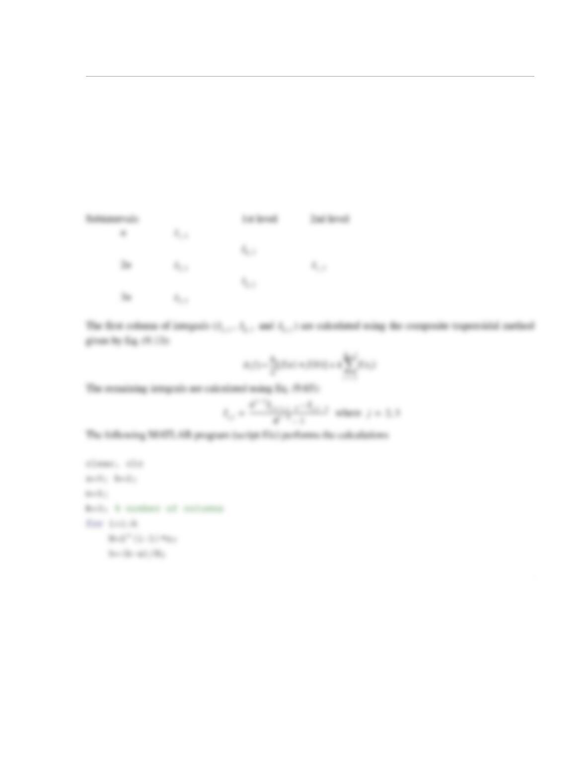
For second-level Romberg integration the integral is calculated with the composite trapezoidal integration

three times using and subintervals, respectively. After that, the second-level Romberg integration

is calculated using the scheme described in Section 9.10:

πx2

2

——-–





xdcos

0

2



n1=

n2n,

3n

2

x=a:h:b;

y=cos(pi*x.^2/2);

% Calculate first column using composite trapezoidal method, Eq. (9.13)

IR(i,1)=h/2*(y(1)+y(N+1))+h*sum(y(2:N));

end

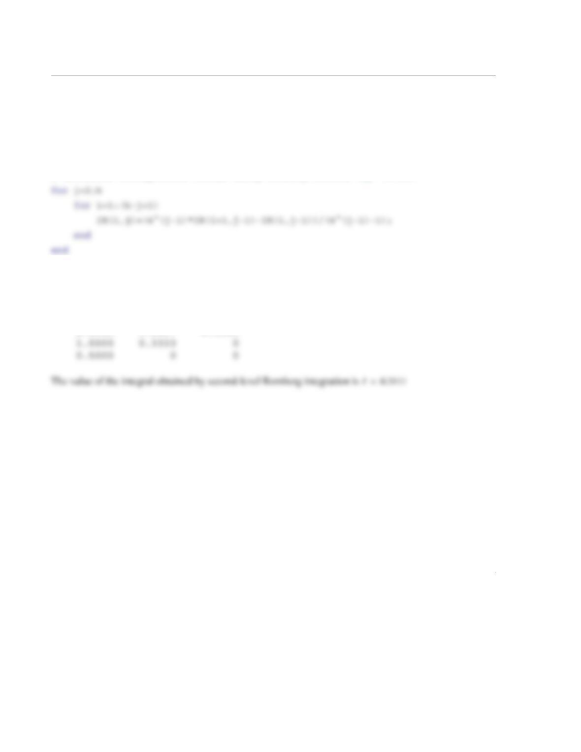
% Calculate extrapolated values using Romberg method, Eq. (9.65)

IR

When the script is executed, the matrix is displayed in the Command Window:

IR =

2.0000 0.6667 0.3111

kk×

IR[]

1

9.16 Evaluate the error integral defined as: at by using four-point Gauss

quadrature.

Solution

The coefficients and Gauss points for forth-order Gauss quadrature are given in Table 9-1 and are valid if

the range of integration is . Because the range of integration in the present problem is , the

integral must be rewritten according to Eq. (9.31):

and

The integration then has the form:

When the script is executed, the value of the integral I appears in the Command Window:

I =

0.995488921128100

erf x() 2

π

——– et2

–td

0

x



=

x2=

1–1,[]

02,[]

x1

2

—–tb a–()ab++[]=

dx 1

2

—–ba–()dt=