3
The listing of the user-defined function ODEsHW10_6 (the system of ODEs in Problem 10.6) that is used in
the solution is:
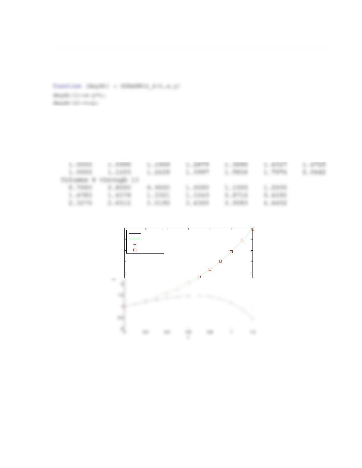
When the program is executed the numerical solution is displayed in the Command Window and the fol-
lowing plot is displayed in the Figure Window:
Answer =
Columns 1 through 7
0 0.1000 0.2000 0.3000 0.4000 0.5000 0.6000
2.5
3
3.5
4
4.5
Exact x
Exact y
Numerical x
Numerical y
4
(b) The ODE in Problem 10.12 is:
from to , with and
The second-order equation is transformed to a syatem of two first-order ODEs.
The the user-defined function Sys2ODEsModEu is used in following program (script file) to solve the
system of ODEs in Problem 10.12:
clear, clc
ab=[0 1.5]; INI=[0 1];
h=0.05;
[x, y, w] = Sys2ODEsRKclas(@ODEsHW10_12,ab,h,INI);
plot(x,y)
xlabel(‘x’); ylabel(‘y’)
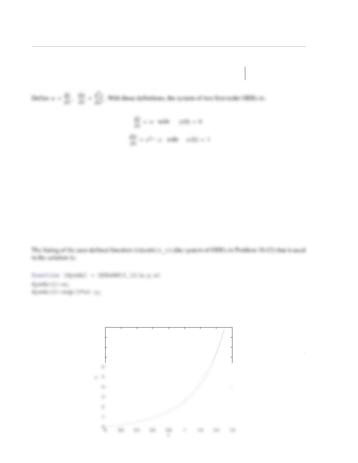
When the program is executed the following plot is displayed in the Figure Window:
d2y
dx2
——––e3xy–=
x0=
x1.5=
y0() 0=
dy
dx
—––
x0=
1=
7
8
9
10
1
10.35 The differential equation for free motion of a spring-mass-damper system is:
where N/m/kg, s–1, , and m/s. Solve the ODE over the interval
s, and plot and (two separate figures on one page) as a function of t.
(a) Use the user-defined function Sys2ODEsModEU that was written in Problem 10.20. For step size use
s.
(b) Use one of MATLAB’s built-in functions for solving ODEs.
Solution
To solve the problem the second-order ODE is rewritten as a system of two first-order ODEs. This is done
by introducing a new variable w, such that:
d2x
dt2
——-– 2γdx
dt
—––k2x++ 0=
k248=
γ0.7=
x0() 0=
dx
dt
—––
t0=
0.2=
0t5≤≤
xt()
dx
dt
—––
0.01
2
h=0.01;
[t, x, w] = Sys2ODEsModEu(@HW10_35aODEs,ab,h,INI);
subplot(2,1,1)
plot(t,x)
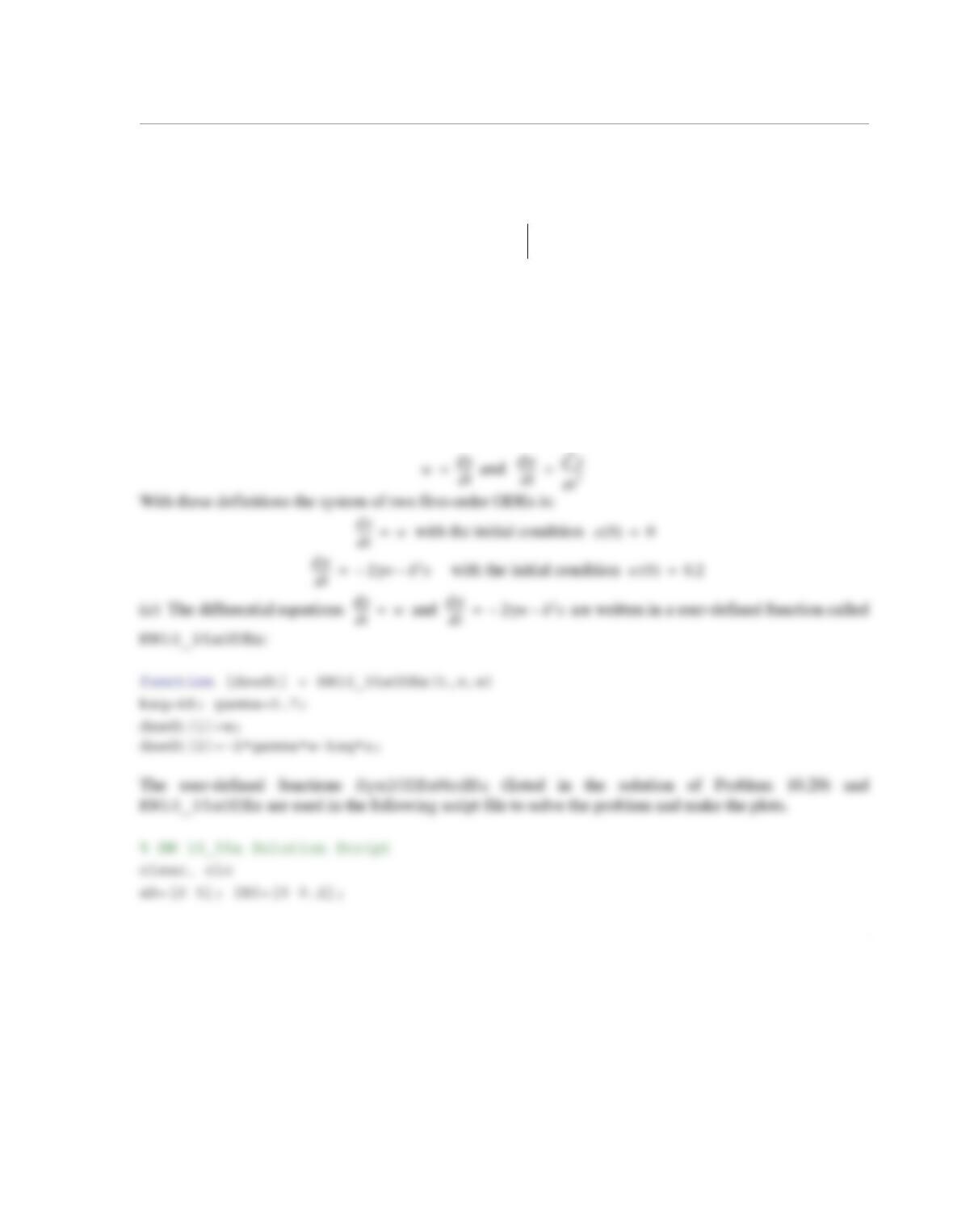
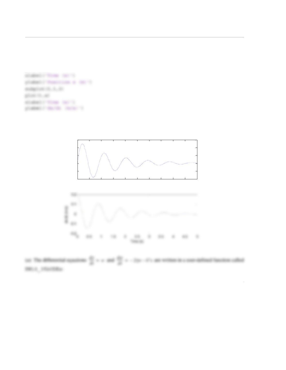
When the script file is executed the following figure that follows is displayed in the Figure Window.
00.5 11.5 22.5 33.5 44.5 5
-0.02
-0.01
0
0.01
0.02
0.03
Time (s)
Position x (m)
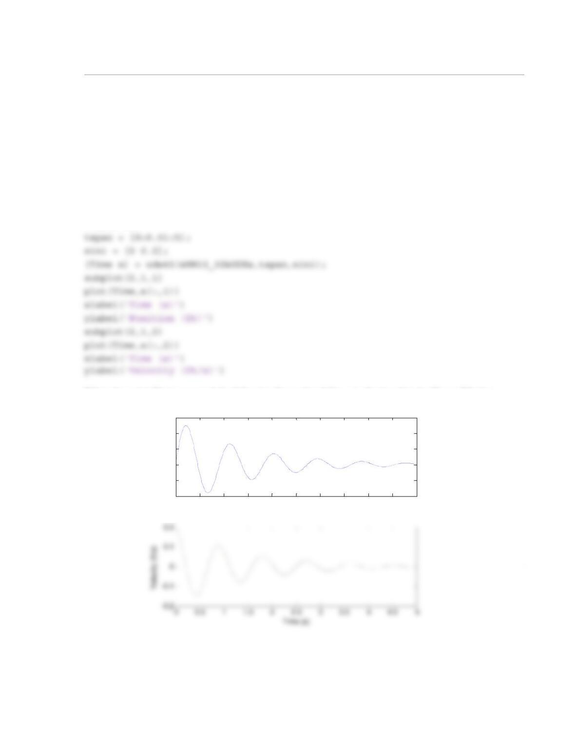
3
function [dxwdt] = HW10_35bODEs(t,x,w)
ksq=48; gamma=0.7;
dxwdt(1)=w;
dxwdt(2)=-2*gamma*w-ksq*x;
MATLAB built-in function ode45 and HW10_35bODEs are used in the following script file to solve the
problem and make the plots.
% HW 10_35b Solution Script
clear, clc
When the script file is executed the following figure that follows is displayed in the Figure Window.
00.5 11.5 22.5 33.5 44.5 5
-0.02
-0.01
0
0.01
0.02
0.03
Time (s)
Position (ft)
1
10.43 The unstable isotope 135Te (atomic weight 135) decays according to:
where s–1, s–1, s–1, and s–1. The instan-
taneous amount of each element is determined from the solution of the following system of ODEs:
Use MATLAB’s built-in functions to find the amount of each element present at the following times. Plot
the results using semilog plots where applicable.
(a) 10-second intervals for the first 5 minutes.
(b) 1000-second intervals for the next 9 hours.
The initial conditions are , .
Solution
The differential equations are written in a user-defined function called ODEsHW10_43:
function dydt = ODEsHW10_43(t, y)
k1=5.78e-3; k2=2.87e-5; k3=2.09e-5; k4=1.1e-12;
135Te k1 135I
135I k2 135Xe
135Xe k3 135Cs
135Cs k4 135Ba
k15.78 10 3–
×=
k22.87 10 5–
×=
k32.09 10 5–
×=
k41.10 10 12–
×=
dTe()
dt
————-– k1Te()–=
dI()
dt
———–k1Te()k2I()–=
dXe()
dt
————-– k2I() k3Xe()–=
dCs()
dt
————-– k3Xe()k4Cs()–=
dBa()
dt
————––k4Cs()=
Te() 6.033 1023
×=
I() Xe() Cs() Ba() 0====
2
figure(2)
semilogy(Time,y(:,2))
xlabel(‘Time (s)’)
ylabel(‘I135’)
figure(3)
semilogy(Time,y(:,3))
xlabel(‘Time (s)’)
When the script file is executed the following figures are displayed in the Figure Window.
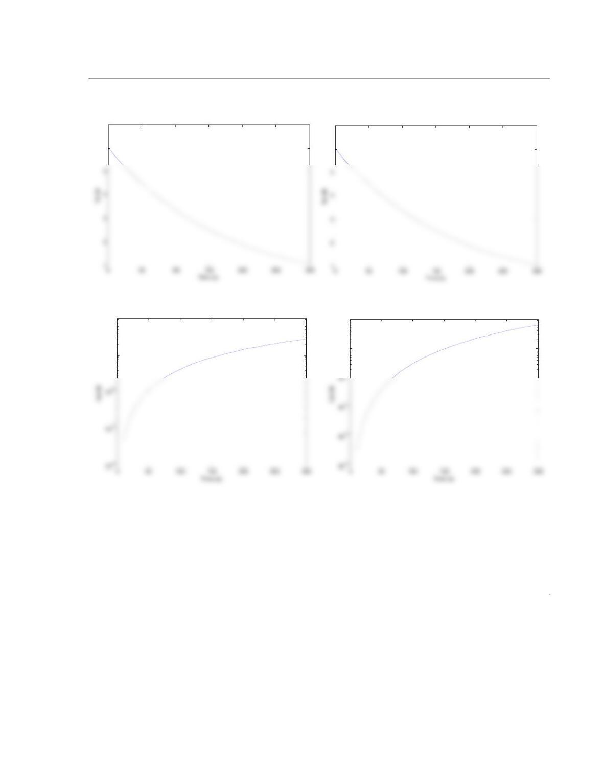
3
6
7x 10²³
6
7x 10²³
1021
1022
1018
1019
4
(b) The user-defined functions ODEsHW10_43 and MATLAB’s built-in function ode45 are used in the
following script file to solve the problem and make the plots.
% HW 10_43b Solution Script
clear, clc
tspan = [0:1000:9*60*60];
yini = [6.022e23 0 0 0 0];
[Time y] = ode45(@ODEsHW10_43,tspan,yini);
figure(1)
107
108
109
Time (s)
5
ylabel(‘Xe135’)
figure(4)
When the script file is executed the following figures are displayed in the Figure Window.
1023.7
1015
1020
1025
6
1023
1024
1024
1013
1014
1015
1016
Ba135