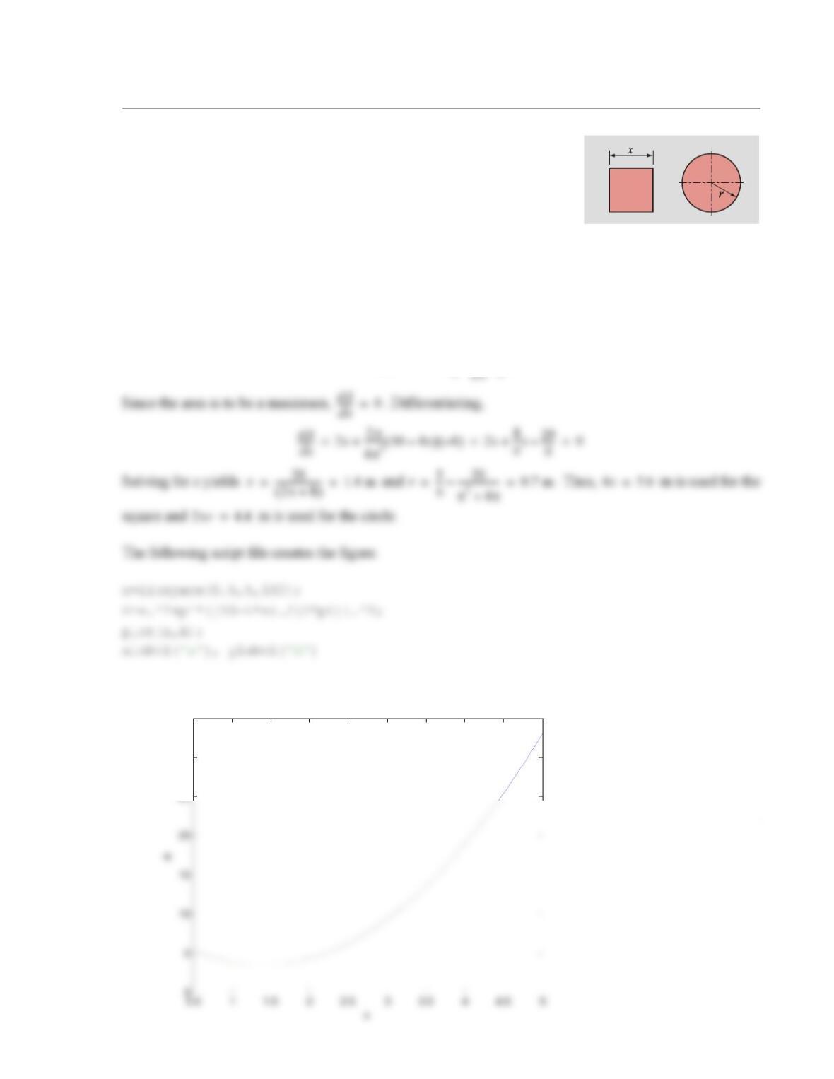
Chapter 2 Homework How much rope should be used for the square and how much for

2.36 Rope with a length of 10 m is to be used to enclose a square area

with side x and a circular area with radius r. How much rope should be

used for the square and how much for the circle if the total area

enclosed by the two shapes is to be a minimum. Plot the total area

enclosed by the two shapes as a function of x, with x varying from 0.5

m to 5 m, and show graphically that the area reaches a minimum at

m.

Solution

Since the sum of the perimeters of the square and circle must add up to 10 m, . The total area

enclosed by the two shapes is . Using the first equation to eliminate r,

When the script is executed, the following figure is displayed:

x1.4=

4x2πr+10=

Ax

2πr2

+=

Ax() x2π10 4x–

—————––

⎝⎠

⎛⎞

2

+=

25

30

35

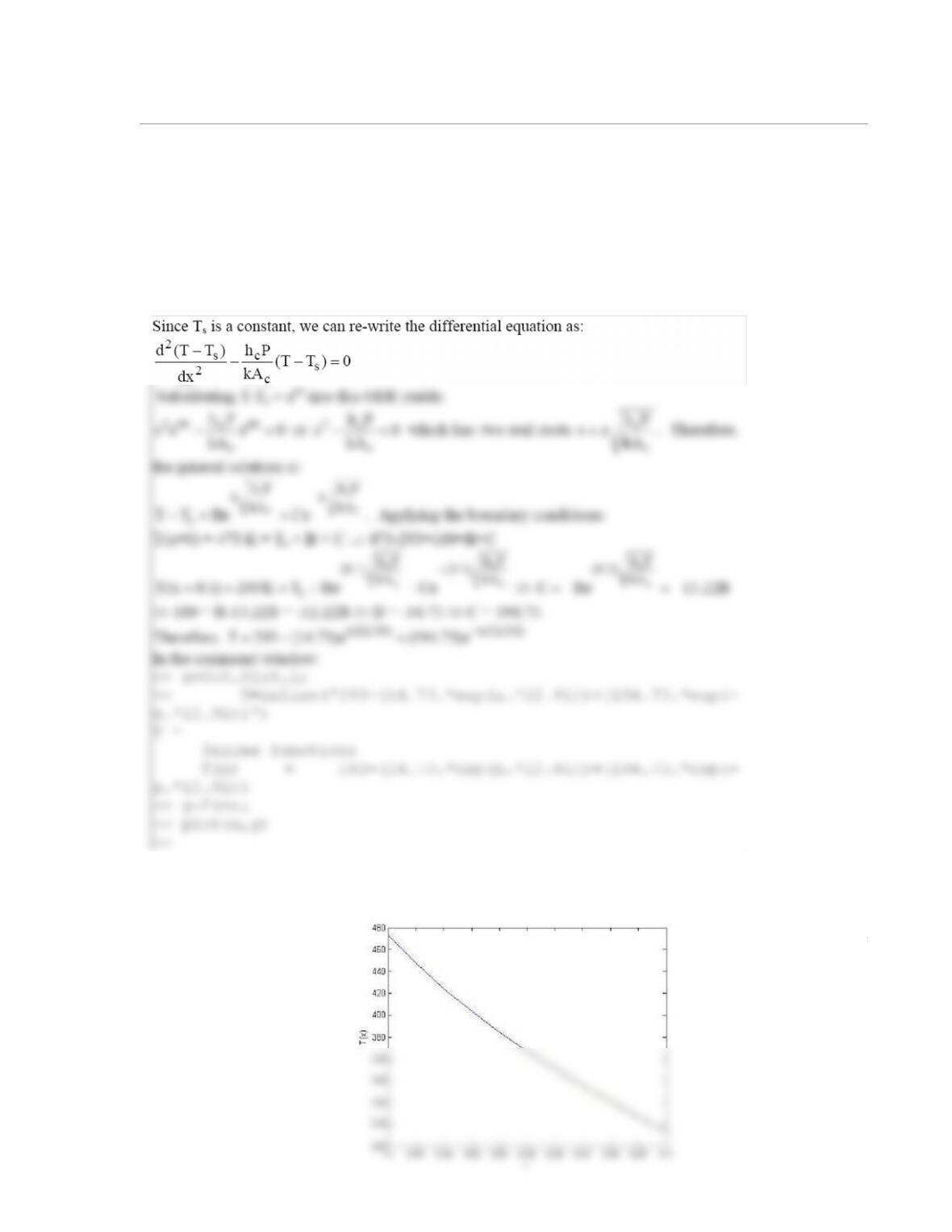
2.37 Solve the ODE for , given that W/m2/K, m,

W/m/K, m2, and K, with K, and K. Plot

using MATLAB.

Solution

d2T

dx2

——–– hcP

kAc

——––TT

s

–()–0=

Tx()

hc40=

P0.016=

k240=

Ac1.6 10 5–

×=

Ts293=

Tx 0=()473=

Tx 0.1=()293=

Tx()

The resulting plot is:

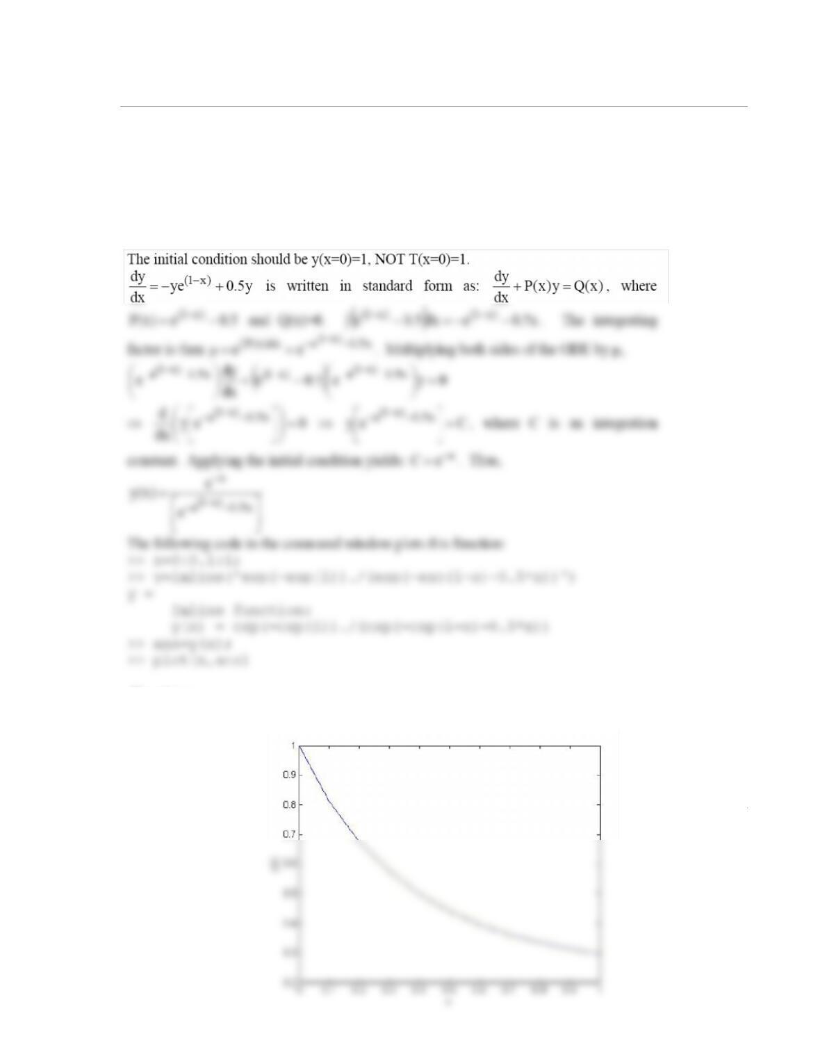
2.38 Solve the ODE with . Use MATLAB to make a plot of ver-

sus x for .

Solution

dy

dx

—––ye 1x–()

–0.5y+=

Tx 0=()1=

yx()

0x1≤≤

The plot is:

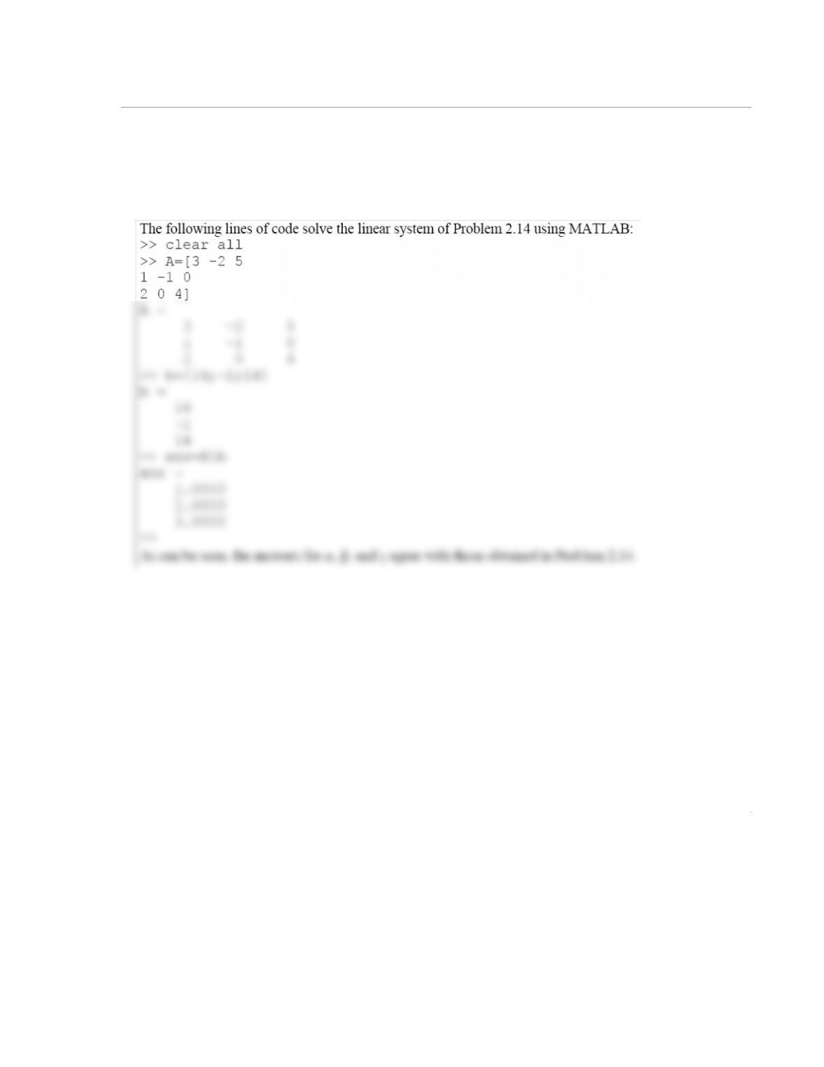
2.39 Solve the system of linear equations in Problem 2.14 for unknowns , , and using MATLAB.

Solution

α

β

γ

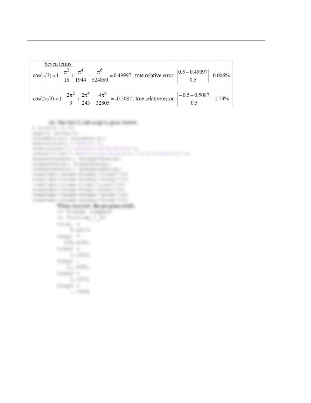
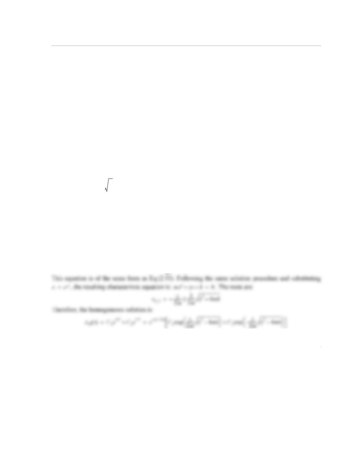
2.40 Approximate the function by using Taylor series expansion about , using three,

five, and seven terms.

(a) In each case calculate the approximated value of the function and the true relative error at

and at .

(b) Using MATLAB, plot the function and the three approximations for .

Solution

yx()cos=

x0=

xπ3⁄=

x2π()3⁄=

0xπ≤≤

2.41 There are mechanical, electrical, and chemical systems that are described by the same mathematics

as second-order, forced, damped harmonic motion. The resulting differential equation obtained after apply-

ing a force balance or conservation of momentum is of the form:

where x is the displacement, t is time, m is the mass, γ is the damping coefficient, k is the restoring force

(spring) constant, is the amplitude of the driving force, and ω is the frequency of the driving force.

(a) Determine the order of the ODE and whether it is linear, nonlinear, homogeneous or non homoge-

neous.

(b) Find the homogeneous solution of the ODE by hand.

(c) Find the particular solution of the ODE by hand. Find after a long time ( ). This is some-

times called the “steady state” response, even though it is actually time varying.

(d) Using MATLAB, plot the maximum amplitude of from the steady state response as a function of

the excitation frequency ω ( rad/s) for N, N/m, and kg, for three values

of γ: , , and N–s/m (three plots on the same figure). Discuss the results. What

happens at when ?

Solution

(a) The highest order derivative that appears in the ODE is second order, so this is a second order ODE.

The coefficients are all constants and the right hand side is a function only of the independent variable t, so

that this is a linear ODE. In standard form, , , , and . Therefore,

this is a non-homogeneous ODE. The given ODE is thus a second order, linear, non-homogeneous ODE.

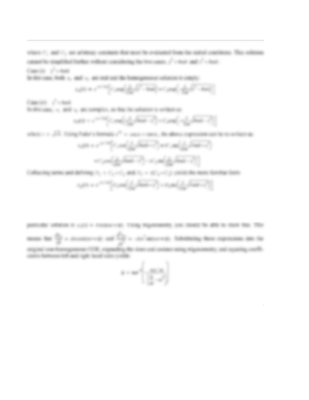
(b) The homogeneous solution is found by setting the right hand side to zero:

md2x

dt2

——-–γdx

dt

—––kx++ A0ωt()sin=

A0

xt()

t∞→

xt()

0ω5≤≤

A01=

k1=

m1=

γ0.5=

γ1.0=

γ2.0=

ωk

m

—–=

γ0=

a3m=

a2γ=

a1k=

rt() A0ωt()sin 0≠=

md2x

——-–γdx

dt

—––kx++ 0=

(c) Since the right hand side does not resemble the homogeneous solution obtained in part (b), a particu-

lar solution can be found by letting , and substituting into the non-homoge-

neous ODE and solving for A and B. An alternative and more compact way of expressing this same

xPt() Aωtφ+()sin=

xPt() Aωt()sin Bωt()cos+=

(d) The maximum amplitude (since the maximum value of sine is 1) is just:

This can be plotted in MATLAB for the parameters specified in this problem. The important point to

remember is that ωt is in radians so that ω has units of radians per second. Frequency ν is measured in

Hertz so that . The following script calculates the maximum amplitude as a function of the

Hertzian frequency and plots it:

AA0

m2k

m

—–ω2

–

⎝⎠

⎛⎞

2ω2γ2

+

——————————————–———–=

νω2π()⁄=

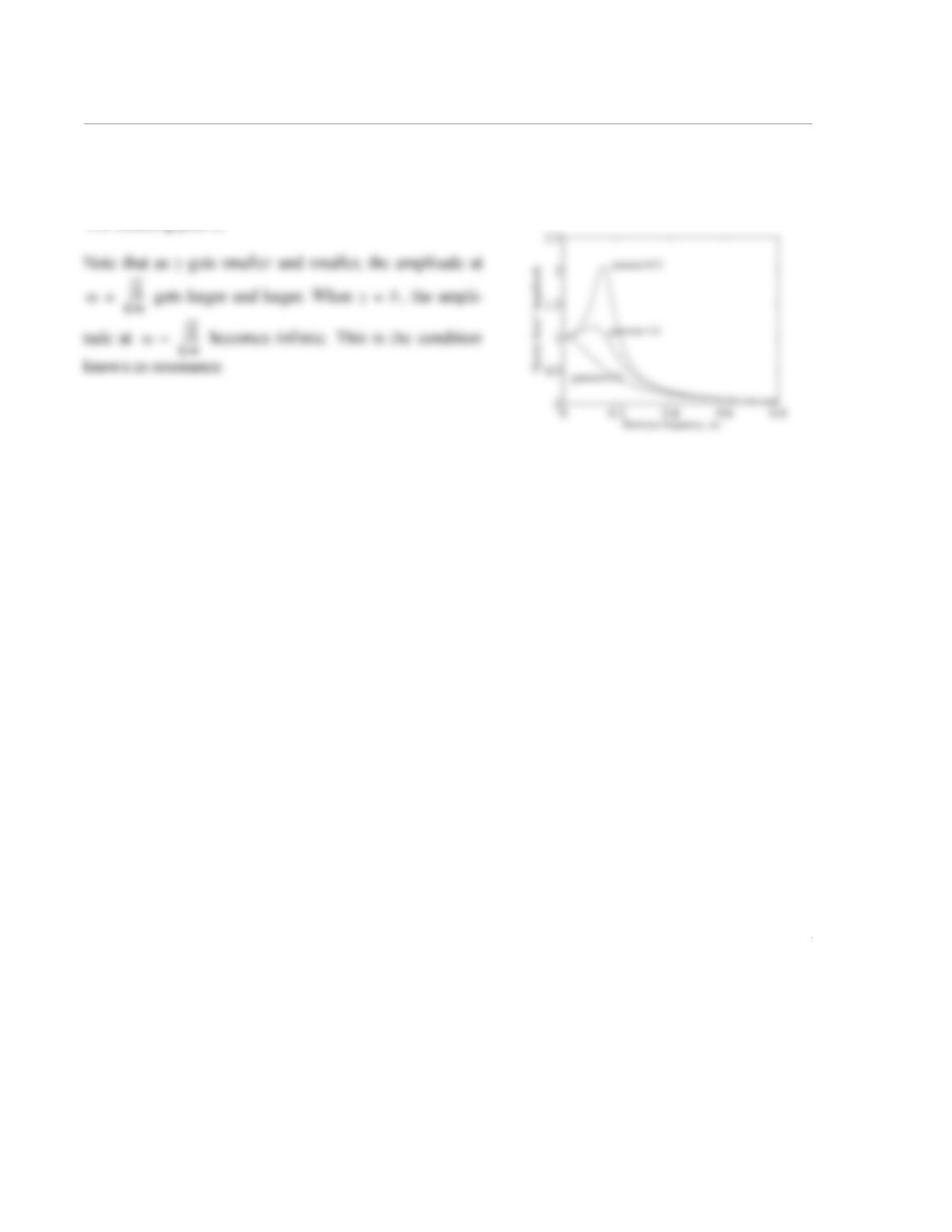
text(0.17,1.1,‘gamma=1.0’)

text(0.03,0.4,‘gamma=2.0’)

The resulting plot is: