1
8.35 The following data for mean velocity near the wall in a fully developed turbulent pipe air flow was
measured [J. Laufer, “The Structure of Turbulence in Fully Developed Pipe Flow,” U.S. National Advisory
Committee for Aeronautics (NACA), Technical Report 1174, 1954]:
y is the distance from the wall, in. is the radius of the pipe, and ft/s. Use the data to calcu-
late the shear stress defined by . lb-s/ft2 is the dynamic viscosity. Note
that will have units of lb/ft2.
(a) Use the user-defined function FirstDerivUneq written in Problem 8.23.
(b) Use MATLAB’s built-in function diff.
Solution
a) The following scripts file uses the user-defined function FirstDerivUneq that was written in Prob-
lem 8.23to solve the problem.
b) The following scripts file uses MATLAB’s built-in function diff to solve the problem.
clear, clc,
meu=3.8E-7;
y/R 0.0030 0.0034 0.0041 0.0051 0.0055 0.0061 0.0071 0.0075 0.0082
0.140 0.152 0.179 0.221 0.228 0.264 0.300 0.318 0.343
u
uU⁄
R4.86=
U9.8=
τ
µdu
dy
—––µU
R
—–du U⁄(
dy R⁄(
—————–
==
µ3.8 10 7–
×=
τ
2
yR=[0.003 0.0034 0.0041 0.0051 0.0055 0.0061 0.0071 0.0075 0.0082];
uU=[0.14 0.152 0.179 0.221 0.228 0.264 0.3 0.318 0.343];
tau=meu*diff(uU)./diff(yR)
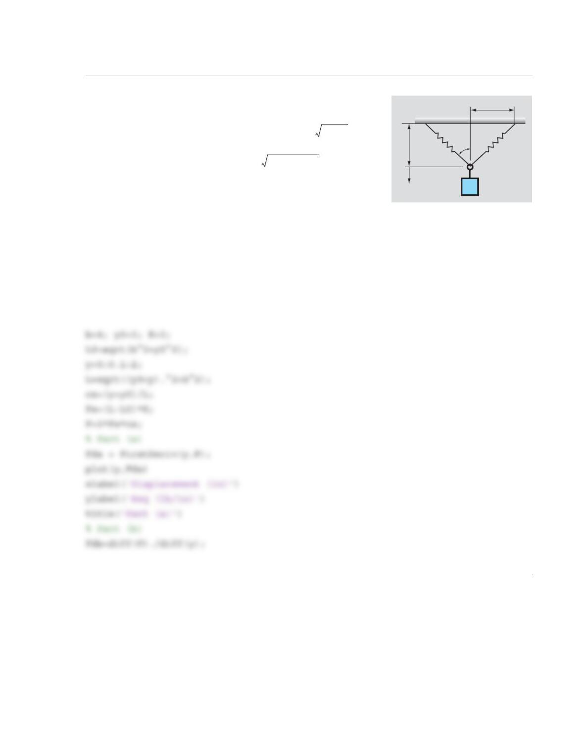
When the script is executed, the following results are displayed in the Command Window, and the figure
that follows is displayed.
1
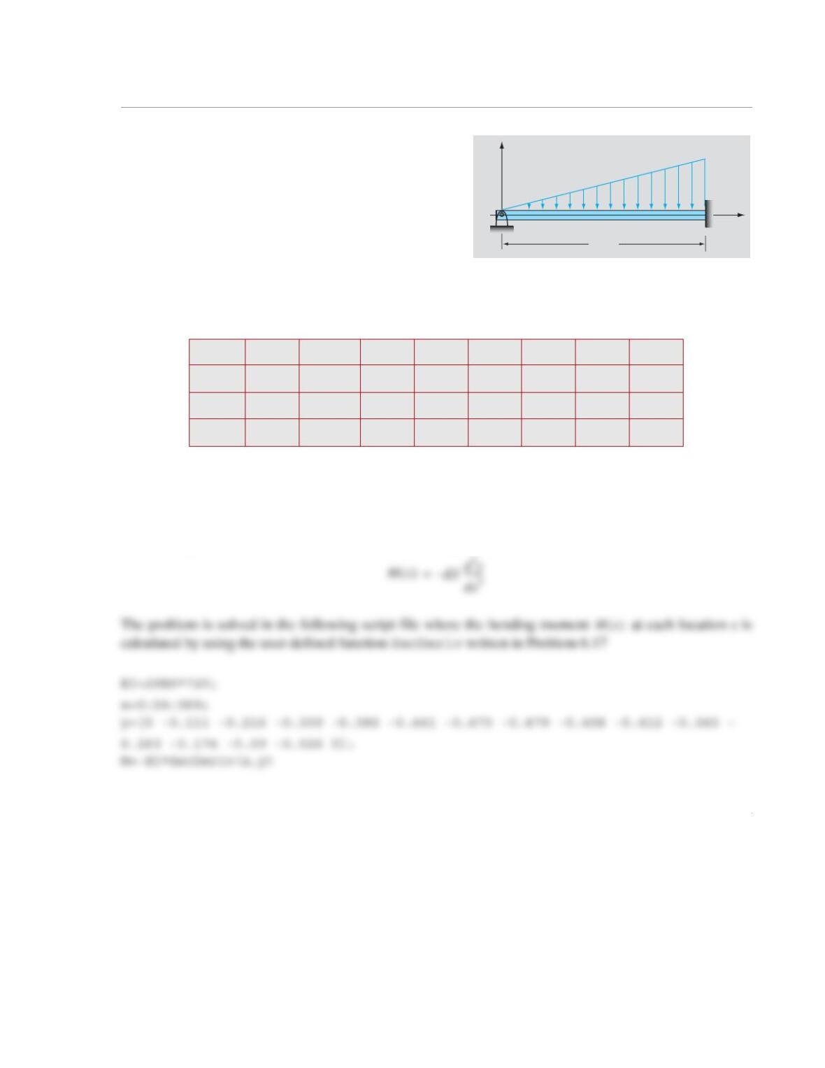
8.36 A 30-ft-long uniform beam is simply supported
at the left end and clamped at the right end. The beam
is subjected to the triangular load shown. The deflec-
tion of the beam is given by the differential equation:
where y is the deflection, x is the coordinate measured
along the length of the beam, is the bending
moment, psi is the elastic modulus, and
in4 is its moment of inertia. The following data is obtained from measuring the deflection of the
beam versus position:
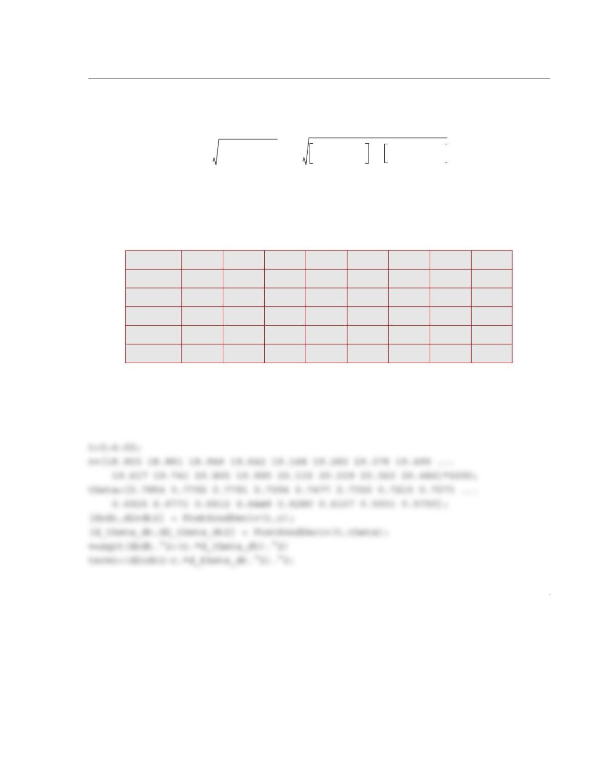
Using the data, determine the bending moment at each location x. Solve the problem by using the
user-defined function SecDeriv written in Problem 8.18. Make a plot of the bending moment diagram
Solution
The bending moment can be solved for from the given ODE:
(in) 024 48 72 96 120 144 168
(in) 0–0.111 –0.216 –0.309 –0.386 –0.441 –0.473 –0.479
(in) 192 216 240 264 288 312 336 360
(in) –0.458 –0.412 –0345 –0.263 –0.174 –0.090 –0.026 0
x
y
q
0
L
d2y
dx2
——––Mx()
EI
———––
=
Mx()
E29 106
×=
I720=
x
y
x
y
Mx()
Mx()
2
When the script file is executed, the following result is displayed in the Command Window:
M =
1.0e+06 *
1
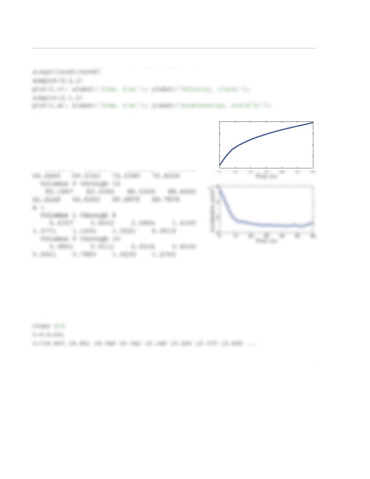
8.37 A radar station is tracking the motion of an aircraft. The recorded distance to the aircraft, r, and the
angle θ during a period of 60 s is given in the following table. The magnitude of the instantaneous velocity
and acceleration of the aircraft can be calculated by:
Determine the magnitudes of the velocity and acceleration at the times given in the table. Plot the velocity
and acceleration versus time (two separate plots on the same page). Solve the problem by writing a pro-
gram in a script file. The program evaluates the various derivatives that are required for calculating the
velocity and acceleration, and then makes the plots. For calculating the derivatives use
(a) the user-defined function FrstScndDeriv that was written in Problem 8.19;
(b) MATLAB’s built-in function diff.
Solution
(a) The following script, in which the user-defined function FrstScndDeriv (written in Problem 8.19)
is used for calculating the derivatives and solve this problem.
t (s) 04812 16 20 24 28
r (km) 18.803 18.861 18.946 19.042 19.148 19.260 19.376 19.495
θ(rad) 0.7854 0.7792 0.7701 0.7594 0.7477 0.7350 0.7215 0.7073
t (s) 32 36 40 44 48 52 56 60
r (km) 19.617 19.741 19.865 19.990 20.115 20.239 20.362 20.484
θ(rad) 0.6925 0.6771 0.6612 0.6448 0.6280 0.6107 0.5931 0.5750
vdr
dt
—-–
2
rdθ
dt
—––
2
+=
d2r
dt2
——-–rdθ
dt
—––
2
–
2
rd2θ
dt2
——-– 2dr
dt
—-– dθ
dt
—––
++=
2
term2=(r.*d2_theta_dt2+2*drdt.*d_theta_dt).^2;
When the program is executed, the following results are dis-
played in the Command Window, and the figure shown on the
right in displayed in the Figure Window.
v =
Columns 1 through 8
24.9465 40.2577 52.0643 58.9943
(b) The following script, in which the MATLAB built-in function diff is used for calculating the deriva-
tives solves this problem. Note that when the diff function is used for calculating the first derivative by
writing drdt=diff(r)./diff(t)and d_theta_dt=diff(theta)./diff(t) it does not calculate
the derivative at the last point. The second derivative is calculated by writing d2rdt2=diff(r,2)/h/h
and d2_theta_dt2=diff(theta,2)/h/h. In this case the second derivative is not calculated in the last
two points.
20
40
60
80
100
Velocity, v(m/s)
3
19.617 19.741 19.865 19.990 20.115 20.239 20.362 20.484]*1000;
theta=[0.7854 0.7792 0.7701 0.7594 0.7477 0.7350 0.7215 0.7073 …
0.6925 0.6771 0.6612 0.6448 0.6280 0.6107 0.5931 0.5750];
[drdt,d2rdt2] = FrstScndDeriv(t,r);
[d_theta_dt,d2_theta_dt2] = FrstScndDeriv(t,theta);
h=t(2)-t(1);
s^2)’);
4
When the program is executed, the following results are dis-
played in the Command Window, and the figure shown on the
right in displayed in the Figure Window.
v =
Columns 1 through 8
32.5524 47.8824 56.0760 61.6806
20
40
60
80
100
Velocity, v(m/s)
1
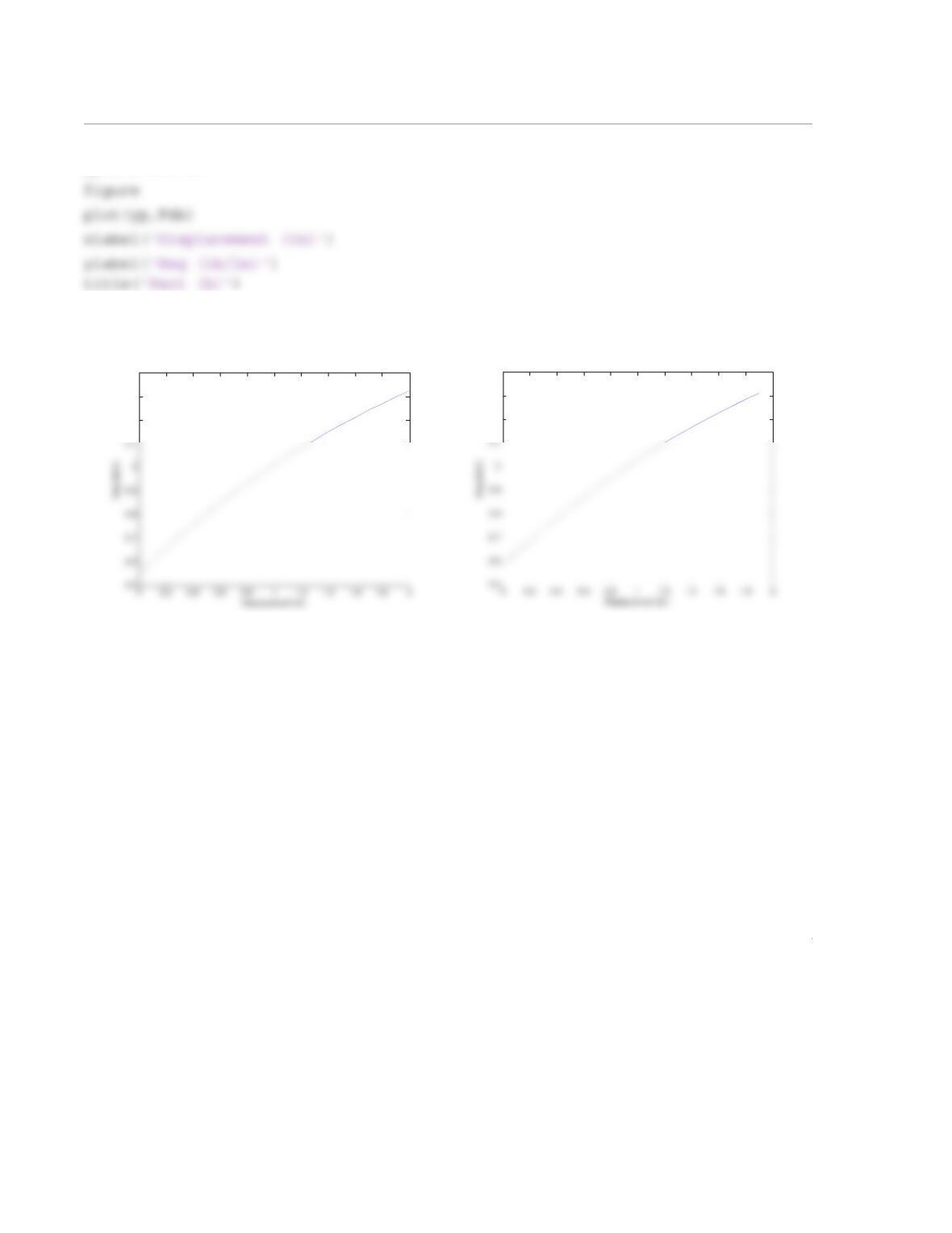
8.38 A scale is made of two springs ( lb/in.) as shown in the
figure ( in., in.). With no weight on the scale
and the length of the spring is given by . As
weights are placed on the scale, it moves down a distance y and the
length of the spring is given by . The force
in each spring is , and the relationship between W
and is . The equivalent spring constant of the scale
is given by . Derive an expression for as in
terms of y and determine the derivative numerically for in. Make a plot of versus y.
(a) Determine the derivative by using the user-defined function FirstDeriv that was written in Prob-
lem 8.17.
(b) Determine the derivative by using MATLAB’s built-in function diff.
Solution
Both parts are solved in the following script file:
W
y
b
K
K
y0θ
K3=
y3=
b4=
y0=
L0
L0b2y0
2
+=
L
Lb
2y0y+()
2
+=
FsKL L
0
–()=
Fs
W2Fθcos=
Keq
Keq
dW
dy
——-–
=
Keq
Keq
0y2≤≤
Keq
2
yp=0:0.1:1.9;
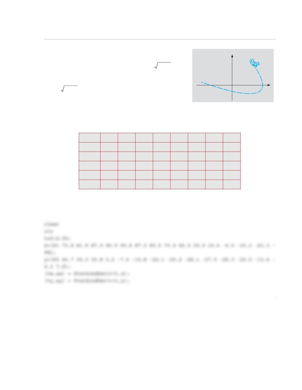
When the script is executed the following figures are displayed:
3.2
3.3
3.4
Part (a)
3.2
3.3
3.4
Part (b)
1
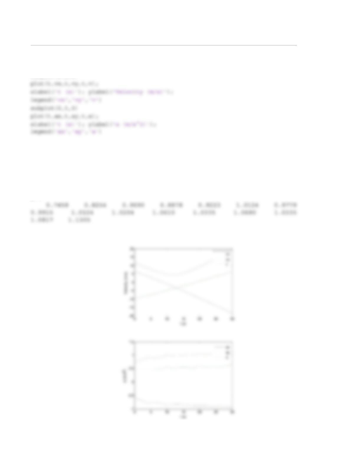
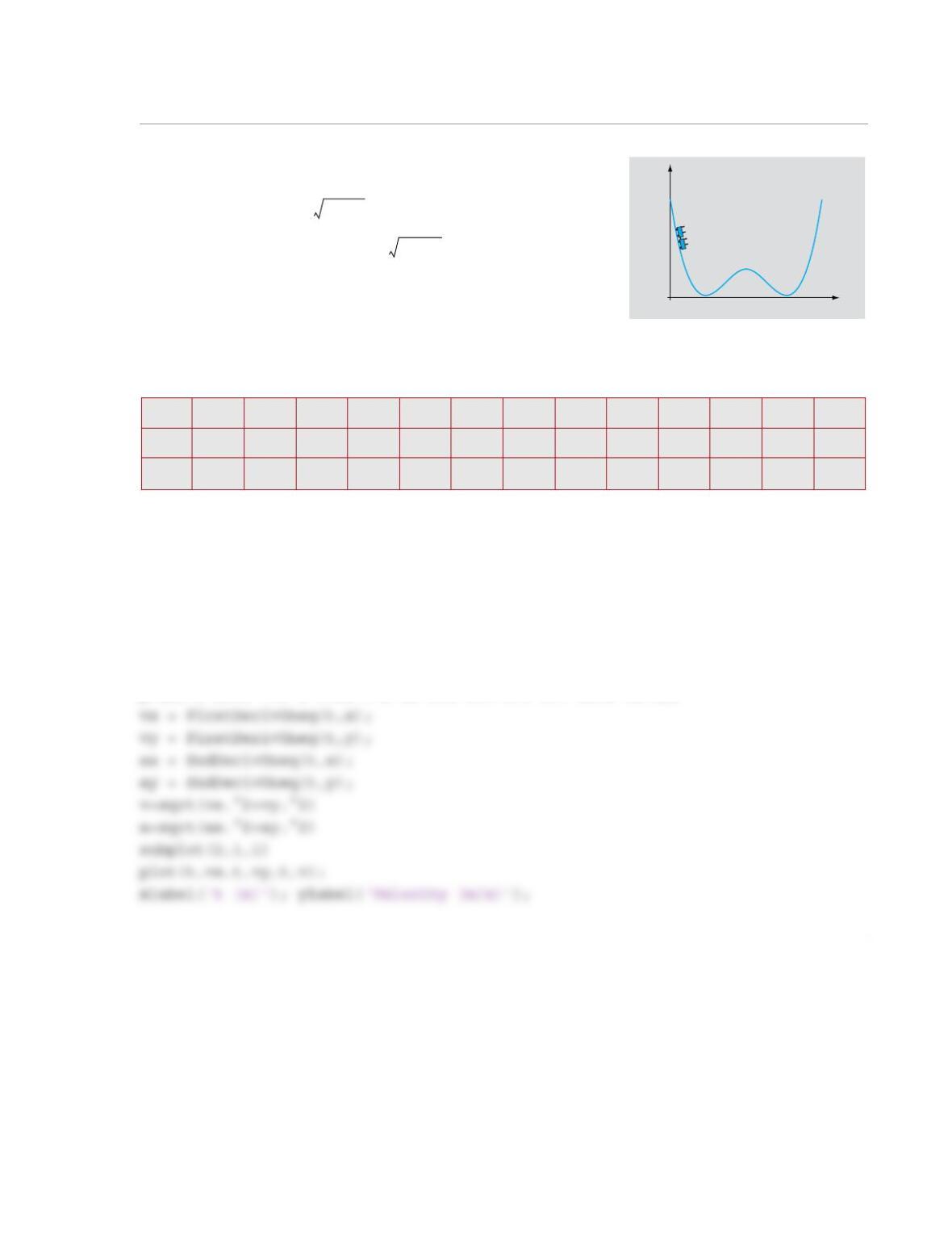
8.39 The position of a squirrel (x and y coordinates) running
around as a function of time, t, is given in the table that follows.
The velocity of the squirrel, v, is given by , where
and . The acceleration of the squirrel, a, is given
by , where and . Write a MAT–
LAB program in a script file that
(a) determines v and a by using the user-defined function Frst-
ScndDeriv that was written in Problem 8.19;
(b) displays a figure with plots of , and v as a function of time (three plots in one figure);
(c) displays a second figure with plots of , and a as a function of time (three plots in one figure)
Solution
The problem is solved in the following script file:
t (s) 0246810 12 14
x (m) 61 72.8 81.9 87.9 90.9 90.8 87.3 80.5
y (m) 65 46.7 30.3 15.8 3.2 –7.4 –15.8 –22.1
t (s) 16 18 20 22 24 26 28 30
x (m) 70.4 56.9 39.9 19.4 –4.6 –32.2 –63.3 –98
y (m) –26.2 –28.1 –27.9 –25.3 –20.5 –13.4 –4.1 7.6
x
y
vv
x
2vy
2
+=
vx
dx
dt
—––
=
vy
dy
dt
—––
=
aa
x
2ay
2
+=
ax
d2x
dt2
——––
=
ay
d2y
∂t2
——––
=
vx
vy
ax
ay
2
v=sqrt(vx.^2+vy.^2)
a=sqrt(ax.^2+ay.^2)
subplot(2,1,1)
When the script is executed, the following results are displayed in the Command Window, and the figures
that follow are displayed in the figure window.
v =
11.6564 10.1270 8.5980 7.1388 5.8451 4.8345 4.4873
4.9609 6.0877 7.6368 9.4011 11.2778 13.2386 15.2370
17.2675 19.3563
a =
1
8.40 The position of the roller coaster cars (x and y coordinates) as
a function of time, t, is given in the table that follows. Determine the
velocity, v, given by , where and , and
the acceleration, a, given by , where and
of the cars. Write a MATLAB program in a script file
that:
(a) Determines v and a as a function of time. (The user-defined functions FirstDerivUneq and Snd-
DerivUneq can be used if Problems 8.23 and 8.24 were solved.)
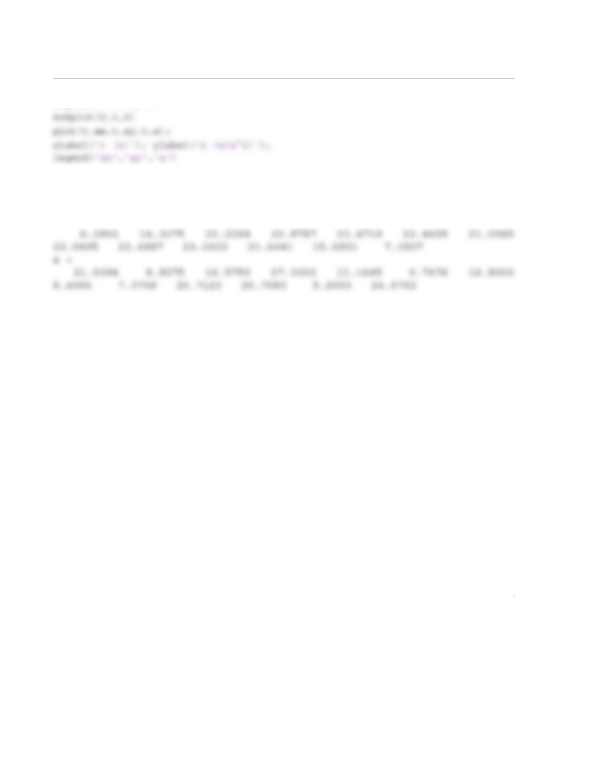
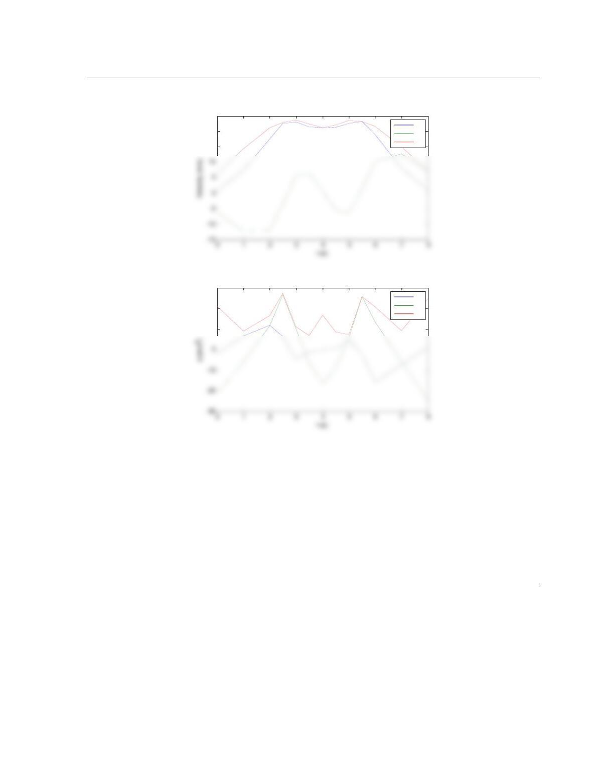
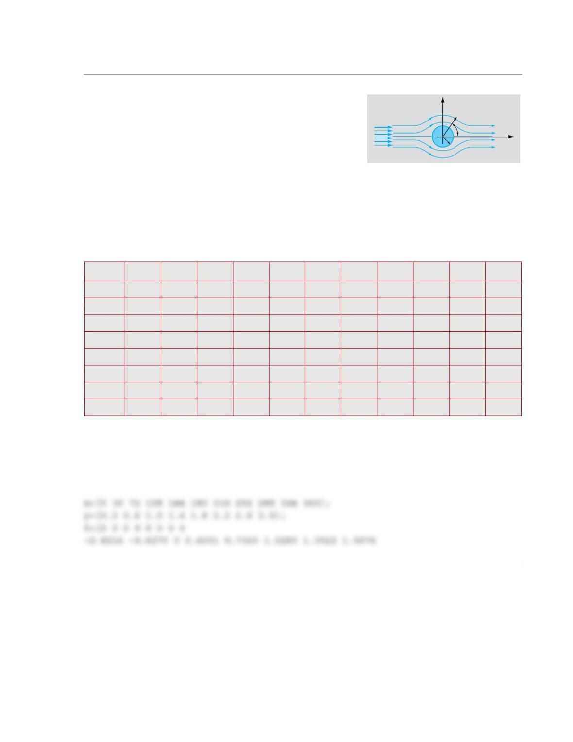
(b) Displays plots of y versus x, v versus x, and a versus x. (Three figures on one page.)
Solution
The problem is solved in the following script file:
clear
clc
t=[0 1 2 2.5 3 3.5 4 4.5 5 5.5 6 7 8 ];
x=[0 4.1 14.9 25.4 37.5 48.4 59 69.6 80.3 92.2 103.5 115.3 119.8];
y=[31.6 22.3 7.1 2 3.54 7.6 10 8.2 4.3 1.8 5.7 21.2 31.1];
(s) 0122.5 33.5 44.5 55.5 678
(m) 04.1 14.9 25.4 37.5 48.4 59 69.6 80.3 92.2 103.5 115.3 119.8
(m) 31.6 22.3 7.1 23.54 7.6 10 8.2 4.3 1.8 5.7 21.2 31.1
x (m)
y (m)
020 40 60 80 100 120
0
5
10
15
20
25
30
35
vv
x
2vy
2
+=
vx
dx
dt
—––
=
vy
dy
dt
—––
=
aa
x
2ay
2
+=
ax
d2x
dt2
——––
=
ay
d2y
∂t2
——––
=
t
x
y
2
legend(‘vx’,‘vy’,‘v’)
When the script is executed, the following results are displayed in the Command Window, and the figures
that follow are displayed in the figure window.
v =
3
15
20
25
vx
vy
v
10
20
30
ax
ay
a
1
8.41 The nondimensional stream function for potential flow
over a cylinder of radius R in an incompressible flow of uniform
velocity U is given in the following table as a function of the non-
dimensional coordinate and the polar angle . The non-
dimensional radial component and the azimuthal compo-
nent of the velocity are given by:
and
Calculate and at every point. Write a MATLAB program that uses two-point central difference
formulas at the interior points and one-sided three-point forward and backward difference formulas at the
endpoints. The user-defined function ParDer can be used instead if Problem 8.25 was solved.
Solution
The user-defined function ParDer from Problem 8.25 can be used here by recognizing that x=θ
and y=r/R. The following script uses the function ParDer from Problem 8.25:
θ=0oθ=36oθ=72oθ=108oθ=144oθ=180oθ=216oθ=252oθ=288oθ=324oθ=360o
r/R=0.2 0–2.8214 –4.5651 –4.5651 –2.8214 02.8214 4.5651 4.5651 2.8214 0
r/R=0.6 0–0.6270 –1.0145 –1.014 –0.6270 00.6270 1.0145 1.0145 0.6270 0
r/R=1.0 00000000000
r/R=1.4 00.4031 0.6522 0.6522 0.4031 0–0.4031 –0.6522 –0.6522 –0.4031 0
r/R=1.8 00.7315 1.1835 1.1835 0.7315 0–0.7315 –1.1835 –1.1835 –0.7315 0
r/R=2.2 01.0260 1.6600 1.6600 1.0260 0–1.0260 –1.6600 –1.6600 –1.0260 0
r/R=2.6 01.3022 2.1070 2.1070 1.3022 0–1.3022 –2.1070 –2.1070 –1.3022 0
r/R=3.0 01.5674 2.5362 2.5362 1.5674 0–1.5674 –2.5362 –2.5362 –1.5674 0
x
y
rθ
R
U
ψ
UR
——-–
rR⁄
θ
urU⁄
uθU⁄
ur
U
—- 1
rR⁄()
————-–
∂ψ
UR
——-–
∂θ
—————-–
=
uθ
U
—-–
∂ψ
UR
——-–
∂rR⁄()
—————––
–=
urU⁄
uθU⁄
2
-4.5651 -1.0145 0 0.6522 1.1835 1.66 2.1070 2.5362
-4.5651 -1.014 0 0.6522 1.1835 1.66 2.1070 2.5362
-2.8214 -0.6270 0 0.4031 0.7315 1.0260 1.3022 1.5674
0 0 0 0 0 0 0 0
end
end
u_r_over_U
u_theta_over_U
When executed, the output is:
u_r_over_U =
-0.4667 -0.0346 0 0.0095 0.0134 0.0154
3
0.3170 0.0235 0 -0.0065 -0.0091 -0.0105 –
0.0113 -0.0117
0.1211 0.0090 0 -0.0025 -0.0035 -0.0040 –
0
-7.4453 -3.5268 -1.2876 -0.9144 -0.7786 -0.7134 –
0.6767 -0.6492
-12.0466 -5.7064 -2.0834 -1.4794 -1.2598 -1.1544 –
1.0953 -1.0507
-12.0491 -5.7064 -2.0827 -1.4794 -1.2598 -1.1544 –
1.0953 -1.0507
-7.4453 -3.5268 -1.2876 -0.9144 -0.7786 -0.7134 –
0.6767 -0.6492
0 0 0 0 0 0 0