1
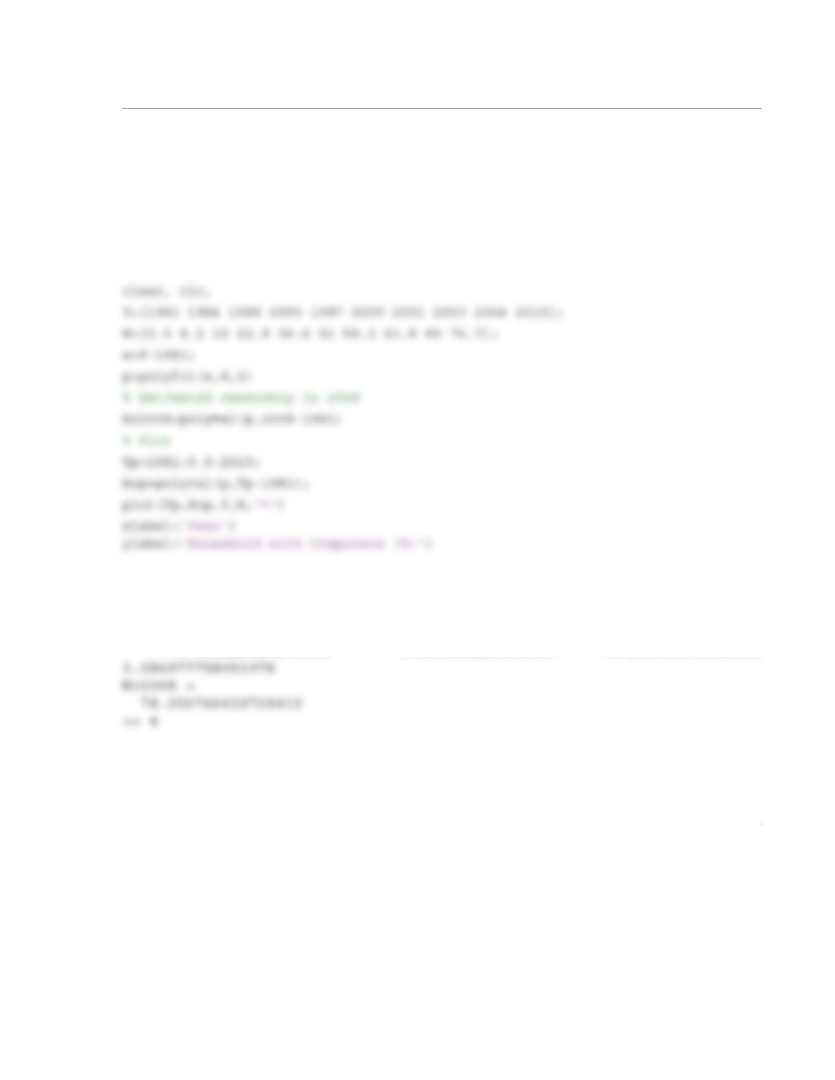
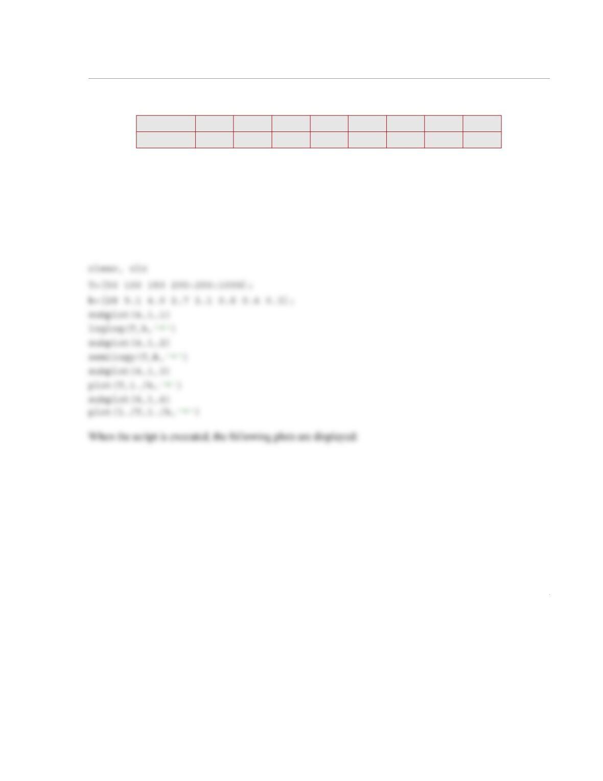
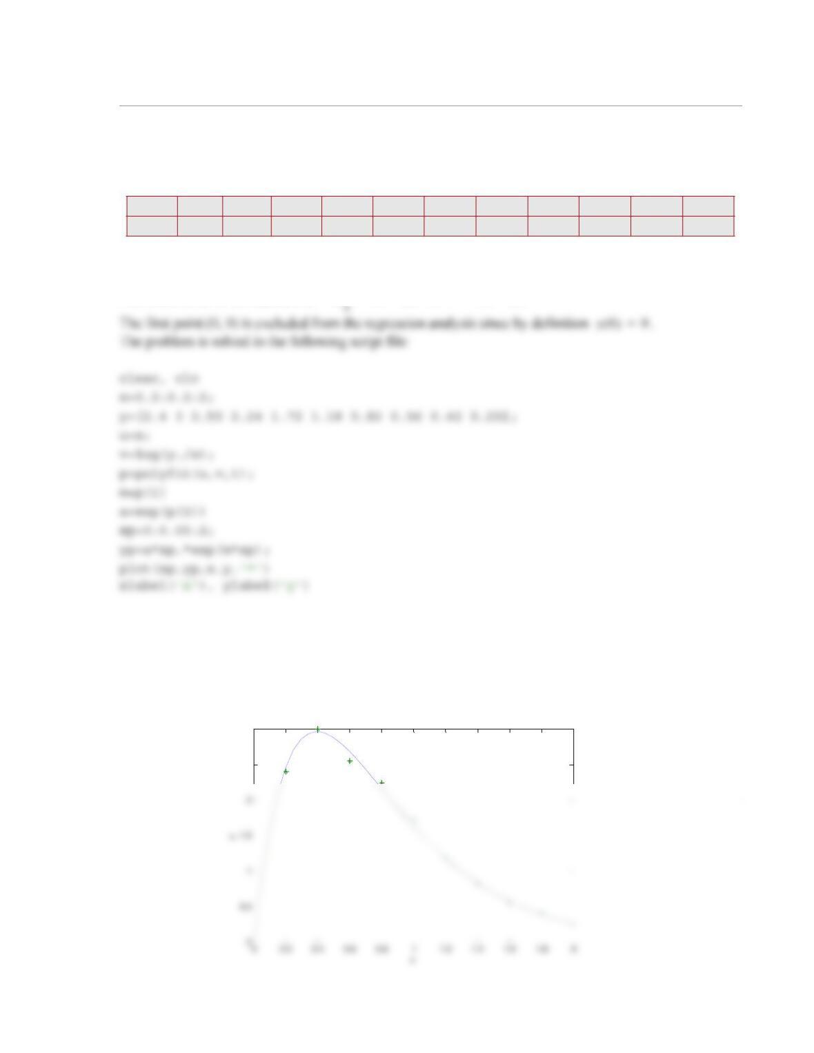
6.32 Use MATLAB’s built-in functions to determine the coefficients of the third-order polynomial,
(where x is the number of years after 1981) that best fits the data in Problem
6.31. Use the polynomial to estimate the percent of computer ownership in 2008 and in 2013. In one fig-
ure, plot the polynomial and the data points.
Solution
The problem is solved in the following script file:
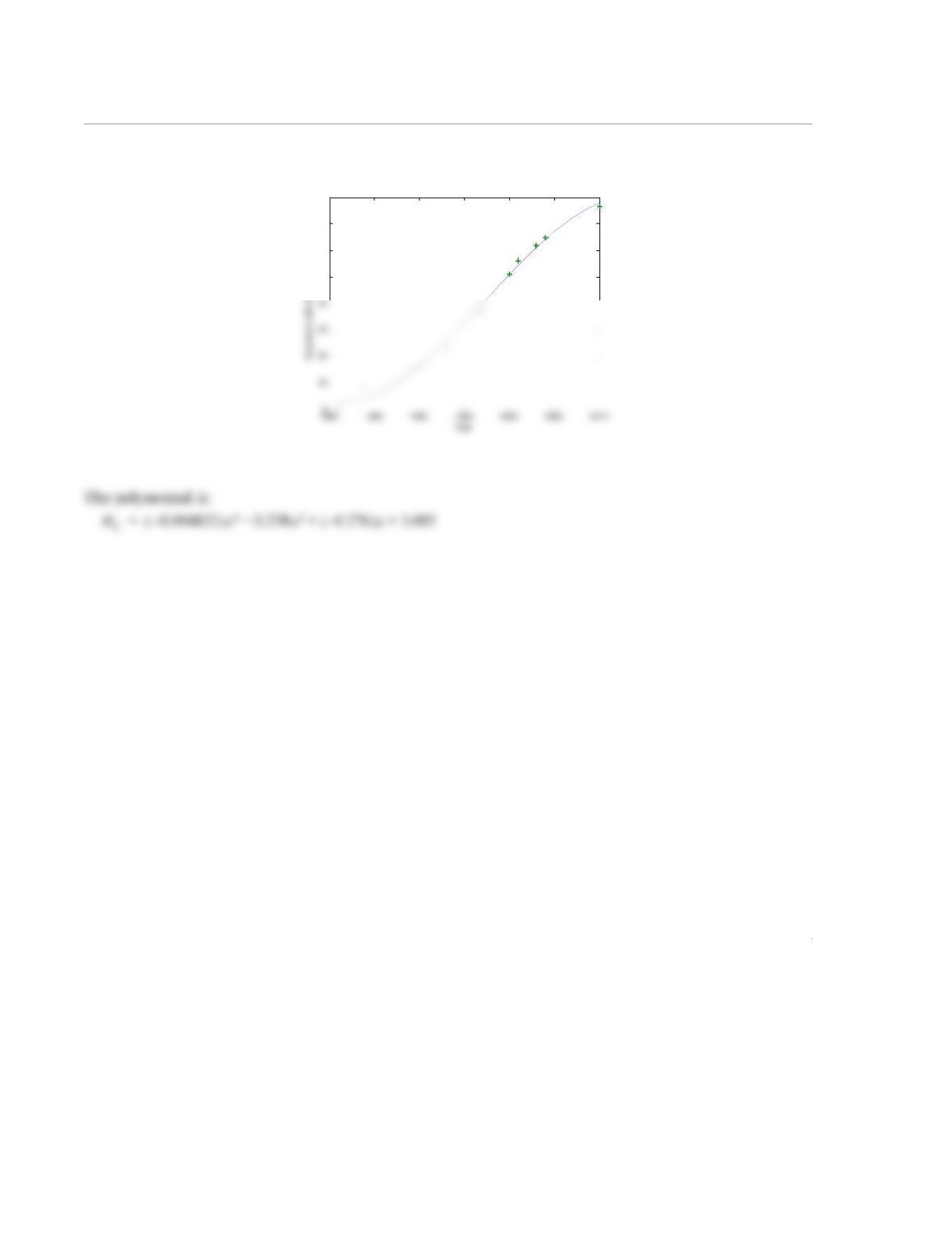
When the script is executed the following results are displayed in the Command Window, and the follow-
ing figure is displayed.
p =
-0.004821523271264 0.238024221835913 -0.275993574014962
HCa3x3a2x2a1xa
0
+++=
2
50
60
70
80
1
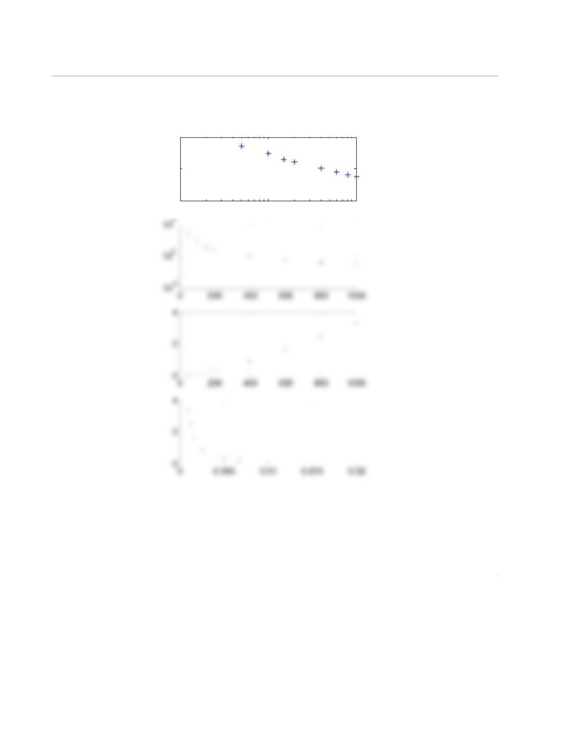
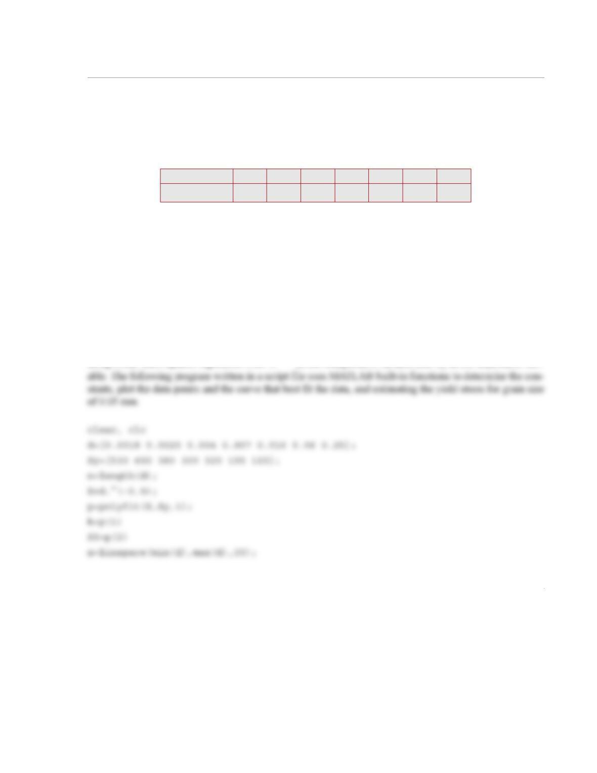
6.33 The following data was obtained when the stopping distance d of a car on a wet road was measured
as a function of the speed v when the brakes were applied:
Determine the coefficients of a quadratic polynomial that best fits the data. Make a
plot that show the data points (asterisk marker) and polynomial (solid line).
(a) Use the user-defined function QuadFit developed in Problem 6.22.
(b) Use MATLAB’s built-in function polyfit.
Solution
(a)
The problem is solved in the following script:
v (mi/h) 12.5 25 37.5 50 62.5 75
d (ft) 20 59 118 197 299 420
da
2v2a1va
0
++=
2
(b)
The problem is solved in the following script:
clear; clc
v=12.5:12.5:75;
d=[20 59 118 197 299 420];
When the script is executed the following figure is displayed.
300
350
400
450
500
300
350
400
450
500
1
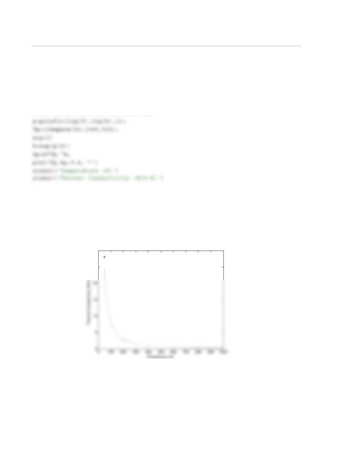
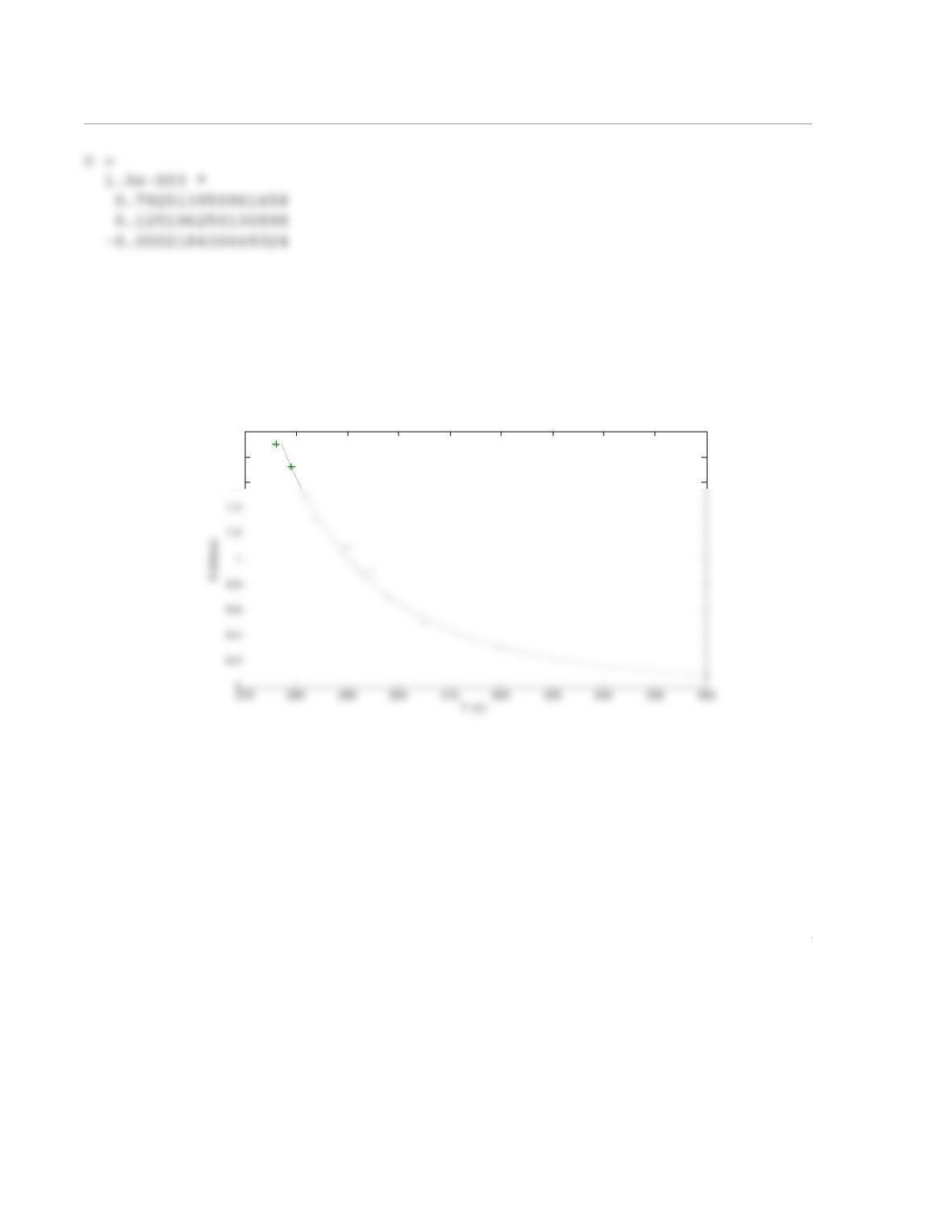
6.34 Measurements of thermal conductivity, k (W/m K), of silicon at various temperatures, T (K), are:
The data is to be fitted with a function of the form . Determine which of the nonlinear equations
that are listed in Table 6-2 can best fit the data and determine its coefficients. Make a plot that shows the
data points (asterisk marker) and the equation (solid line).
Solution
First, the following four plots are made. k vs. T on a log-log plot. k vs. T on a log k (vertical) linear T (hor-
izontal) axes. 1/k vs. T with linear axes. 1/k vs. 1/T with linear axes.
(K) 50 100 150 200 400 600 800 1000
(W/m K) 28 9.1 4.0 2.7 1.1 0.6 0.4 0.3
T
°
k
kfT()=
2
In the top figure the data points appear to fit a straight line. This means that equation of the form:
101102103
10-2
100
102
kbT
m
=
25
30
will best fit the data points.
The constants b and m are then determined by:
clear, clc
T=[50 100 150 200:200:1000];
k=[28 9.1 4.0 2.7 1.1 0.6 0.4 0.3];
When the script is executed the following values of the constants are displayed in the Command Window,
and the following figure is displayed:
m =
-1.494037745708517
b =
8.441641522899816e+03
1
6.35 Thermistors are resistors that are used for measuring temperature. The relationship between temper–
ature and resistance is given by the Steinhart-Hart equation:
where T is the temperature in degrees Celsius, R is the thermistor resistance in , and , , and , are
constants. In an experiment for characterizing a thermistor, the following data was measured:
Determine the constants , , and such that the Steinhart-Hart equation will best fit the data.
Solution
The problem is solved by using the user-defined function NonLinCombFit written in Homework Problem
6.26.
The problem is solved in the following script file. When the program is executed the value of the constants
is displayed in the Command Window. The program create also a figure that display the equation and the
data points.
(C) 360 320 305 298 295 290 284 282 279 276
(Ω)950 3100 4950 6960 9020 10930 13100 14950 17200 18950
1
T273.15+
————————-–C1C2R()ln C3R()ln3
++=
Ω
C1
C2
C3
T
R
C1
C2
C3
2
Thus, the constants are:
The figure is:
C10.79251 10 3–
×=C20.1252 10 3–
×=C30.21843–10
6–
×=
1.6
1.8
2x 10⁴
1
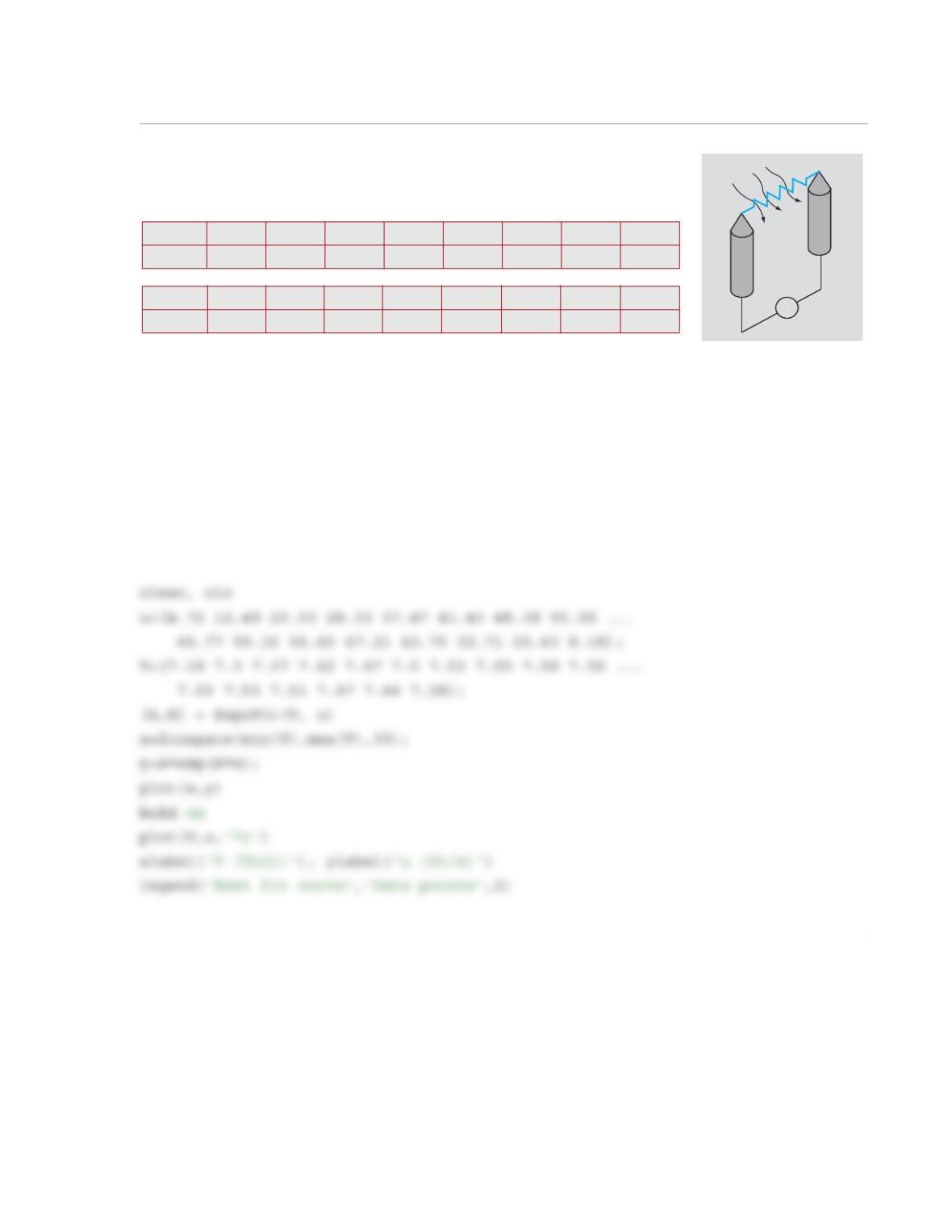
6.36 A hot-wire anemometer is a device for measuring flow velocity, by mea-
suring the cooling effect of the flow on the resistance of a hot wire. The follow-
ing data are obtained in calibration tests:
Determine the coefficients of the exponential funct ion that best fit
the data.
(a) Use the user-defined function ExpoFit developed in Problem 6.20.
(b) Use MATLAB built-in functions.
In each part make a plot that shows the data points (asterisk marker) and the equation (solid line).
Solution
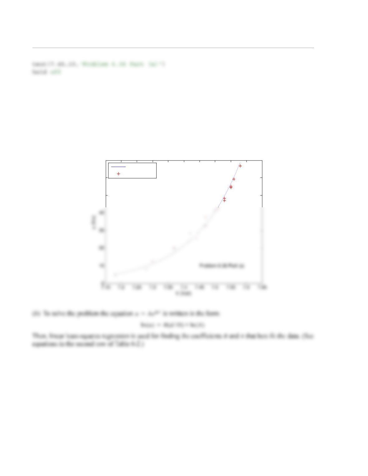
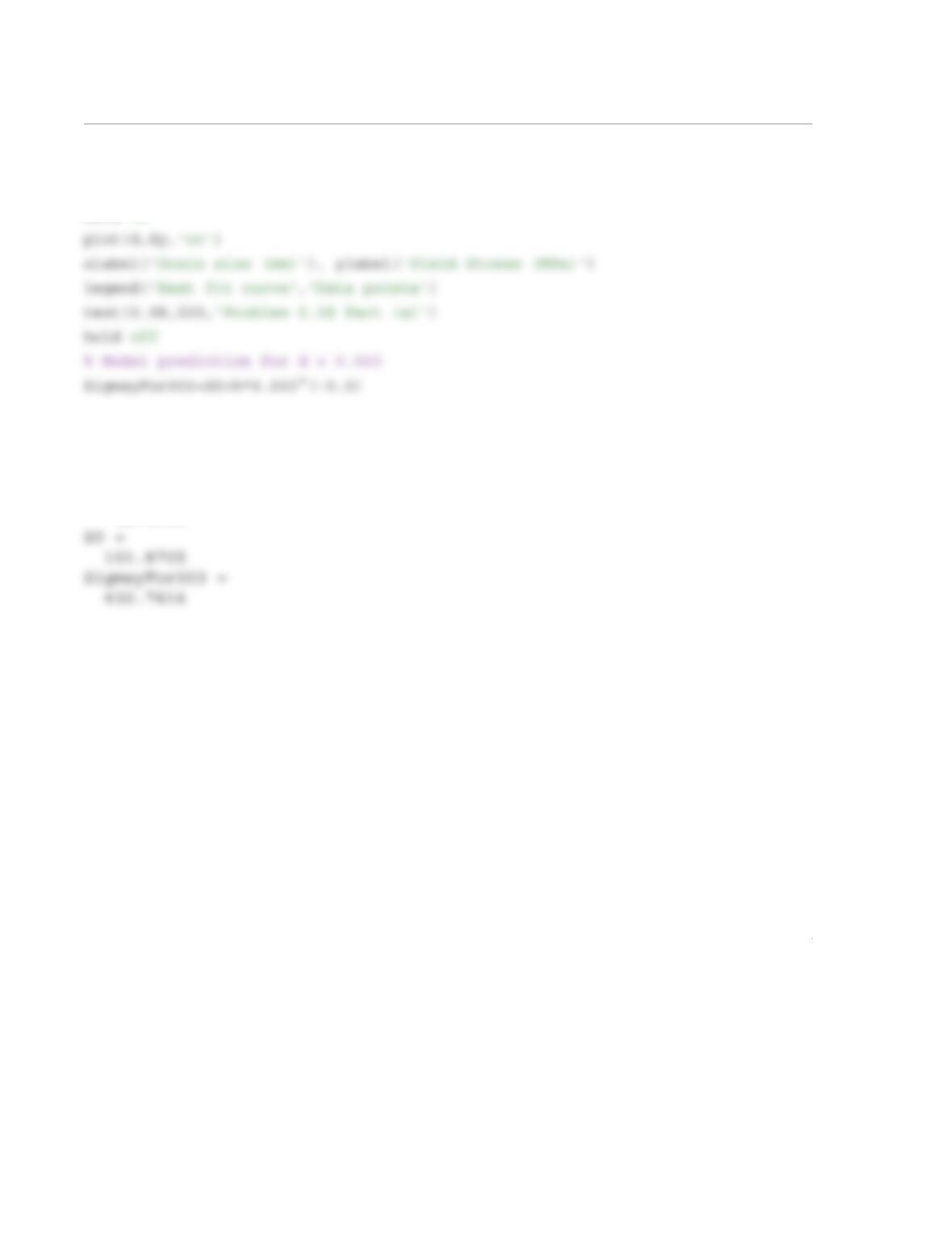
(a) The user-defined function ExpoFit that was developed in Problem 6-20 fits an exponential function
of the form to a given set of data points. The following program written in a scri pt file uses
ExpoFit to determine the constants and plot the data points and the curve that best fit the data.
u (ft/s) 4.72 12.49 20.03 28.33 37.47 41.43 48.38 55.06
V (Volt) 7.18 7.3 7.37 7.42 7.47 7.5 7.53 7.55
u (ft/s) 66.77 59.16 54.45 47.21 42.75 32.71 25.43 8.18
V (Volt) 7.58 7.56 7.55 7.53 7.51 7.47 7.44 7.28
I
u
uAe
BV
=
ybe
mx
=
2
When the program is executed, the following values of B and A are displayed in the Command W indow,
and the figure that follows is displayed in the Figure Window.
A =
2.4825e-020
B =
6.5133
50
60
70
Best fit curve
Data points
3
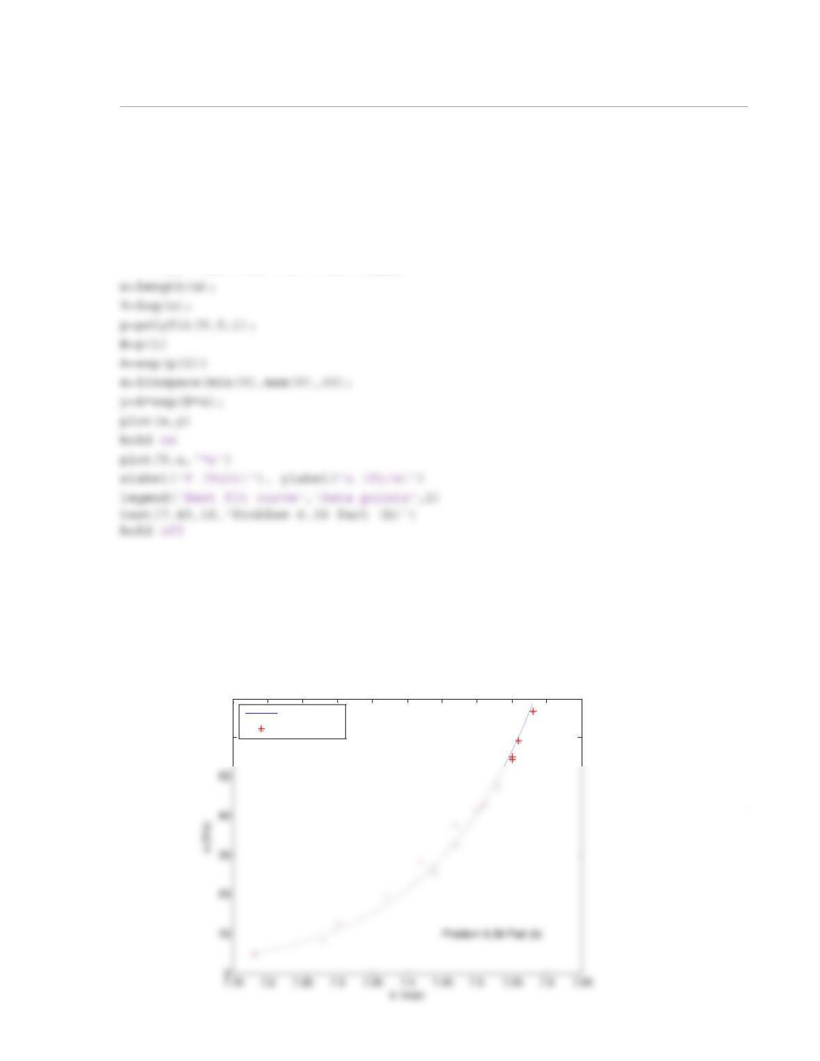
The following program written in a script file uses MATLAB built-in functions to determine the con-
stants and plot the data points and the curve that best fit the data.
clear all
u=[4.72 12.49 20.03 28.33 37.47 41.43 48.38 55.06 …
66.77 59.16 54.45 47.21 42.75 32.71 25.43 8.18];
V=[7.18 7.3 7.37 7.42 7.47 7.5 7.53 7.55 7.58 7.56 …
7.55 7.53 7.51 7.47 7.44 7.28];
When the program is executed, the following values of B and A are displayed in the Command Window,
and the figure that follows is displayed in the Figure Window.
B =
6.5133
A =
2.4825e-020
60
70
Best fit curve
Data points
1
6.37 The data given is to be curve-fitted with the equation . Transform the equation to a linear
form and de termine the constants a and m by using linear least-square regression. (Hint: substi tute
and .) Make a plot that shows the points (circle markers) and the equation (solid line).
Solution
The linear form of the equation is: or
When the script is executed the values of m and a are displayed in the Command Window, and the follow-
ing figure is displayed in the Figure Window.
m =
-2.5184
a =
20.2564
x00.2 0.4 0.6 0.8 1.0 1.2 1.4 1.6 1.8 2.0
y02.40 3.00 2.55 2.24 1.72 1.18 0.82 0.56 0.42 0.25
yaxe
mx
=
vyx⁄()ln=
ux=
y
—ln mx aln+=
vmu aln+=
2.5
3
1
6.38 The yield stress of many metals, , varies with the size of the grains. Often, the relationship
between the grain size, d, and the yield stress is modeled with the Hall–Petch equation:
The following are results from measurements of average grain size and yield stress:
(a) Determine the constants and k such that the Hall–Petch equation will best fit the data. Plot the data
points (circle markers) and the Hall–Petch equation as a solid line. Use the Hall–Petch equation to esti-
mate the yield stress of a specimen with a grain size of 0.003 mm.
(b) Use the user-defined function QuadFit from Problem 6.22 to find the quadratic function that best fits
the data. Plot the data points (circle markers) an d the quadratic equation as a solid line. Use the qua-
dratic equation to estimate the yield stress of a specimen with a grain size of 0.003 mm.
Solution
(a) The coefficients and k that best fit the data in the equation are determined by
using linear least-squares regression with as the independent variable and as the dependent vari-
d (mm) 0.0018 0.0025 0.004 0.007 0.016 0.060 0.25
(MPa) 530 450 380 300 230 155 115
σy
σyσ0kd
1
2
—–
–
+=
σy
σ0
σ0
σyσ0kd
1
2
—–
–
+=
d
1
2
—–
–
σy
2
y=S0+k*x.^(-0.5);
plot(x,y)
hold on
When the program is executed, the values and k and the prediction for grain size of 0.003 mm are dis-
played in the Command Window. The figure that follows is displayed in the Figure Window.
k =
18.0130
σ0