Chapter 3 Homework This Iteration Function Used The Following Mat lab

2

Con=w/(360*L*E*I);

y=@(x) Con*x*(7*L^4-10*L^2*x^2+3*x^4);

yd=@ (x) Con*(7*L^4-10*L^2*3*x^2+3*5*x^4);

ydd=@ (x) Con*(-10*L^2*3*2*x+3*5*4*x^3);

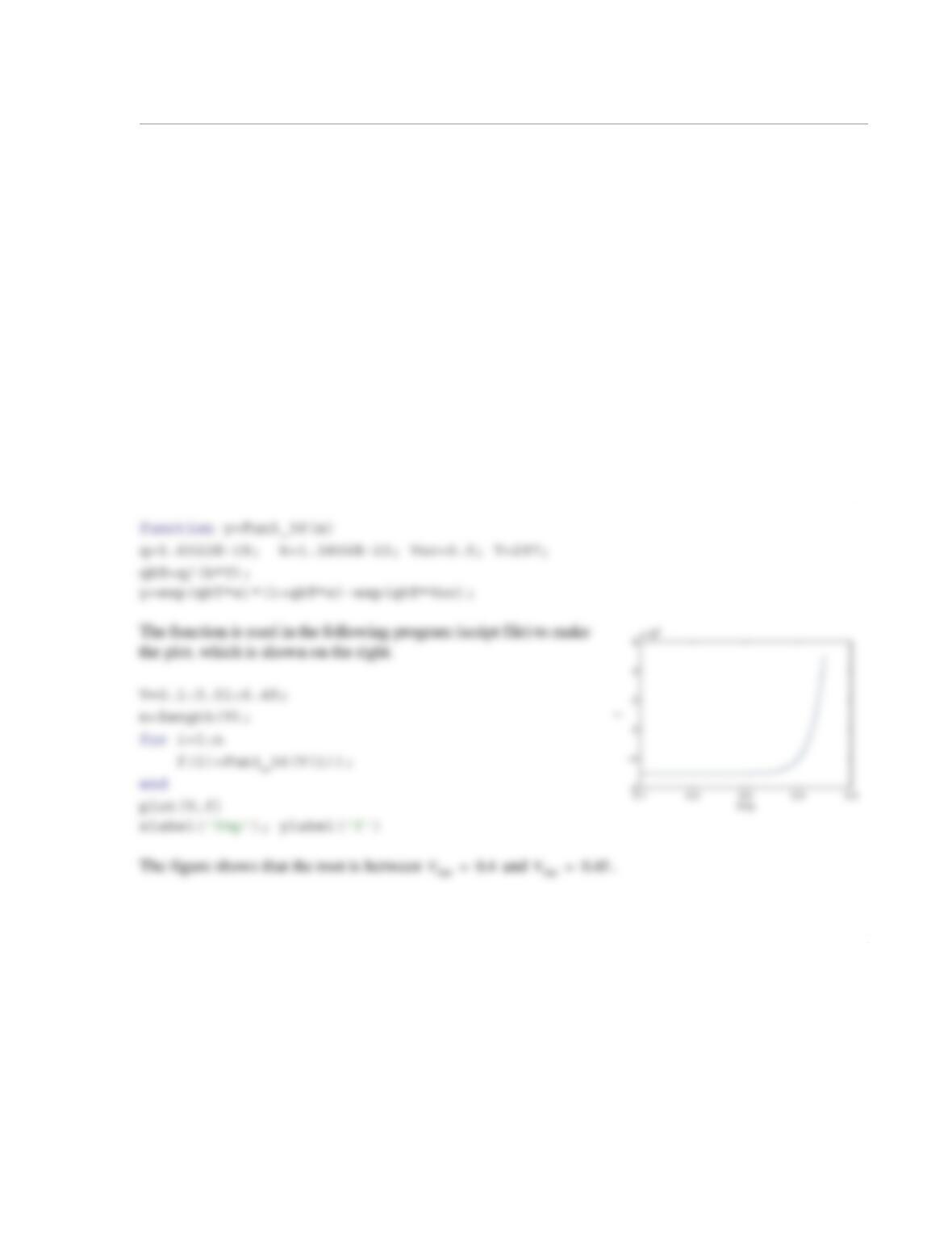
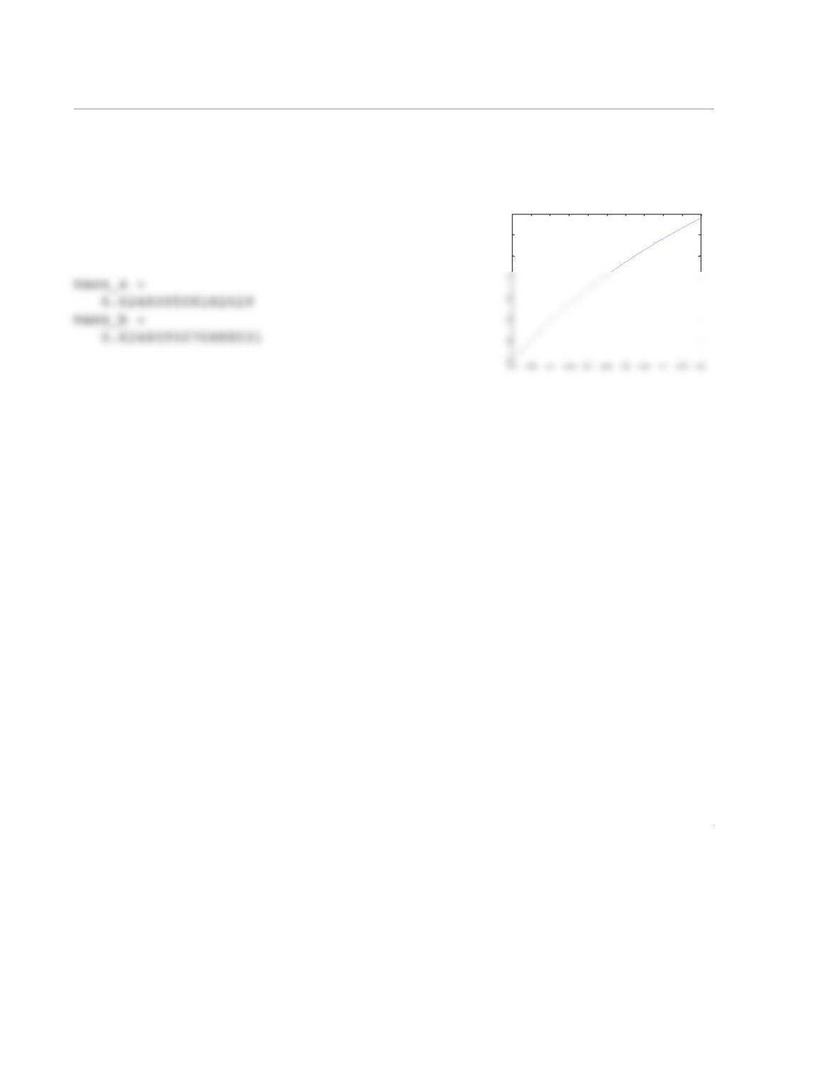
When the script file is executed the following results are displayed in the Command Window:

Part (a)

xMax_a =

2.0773

yMax_a =

0.0090

1

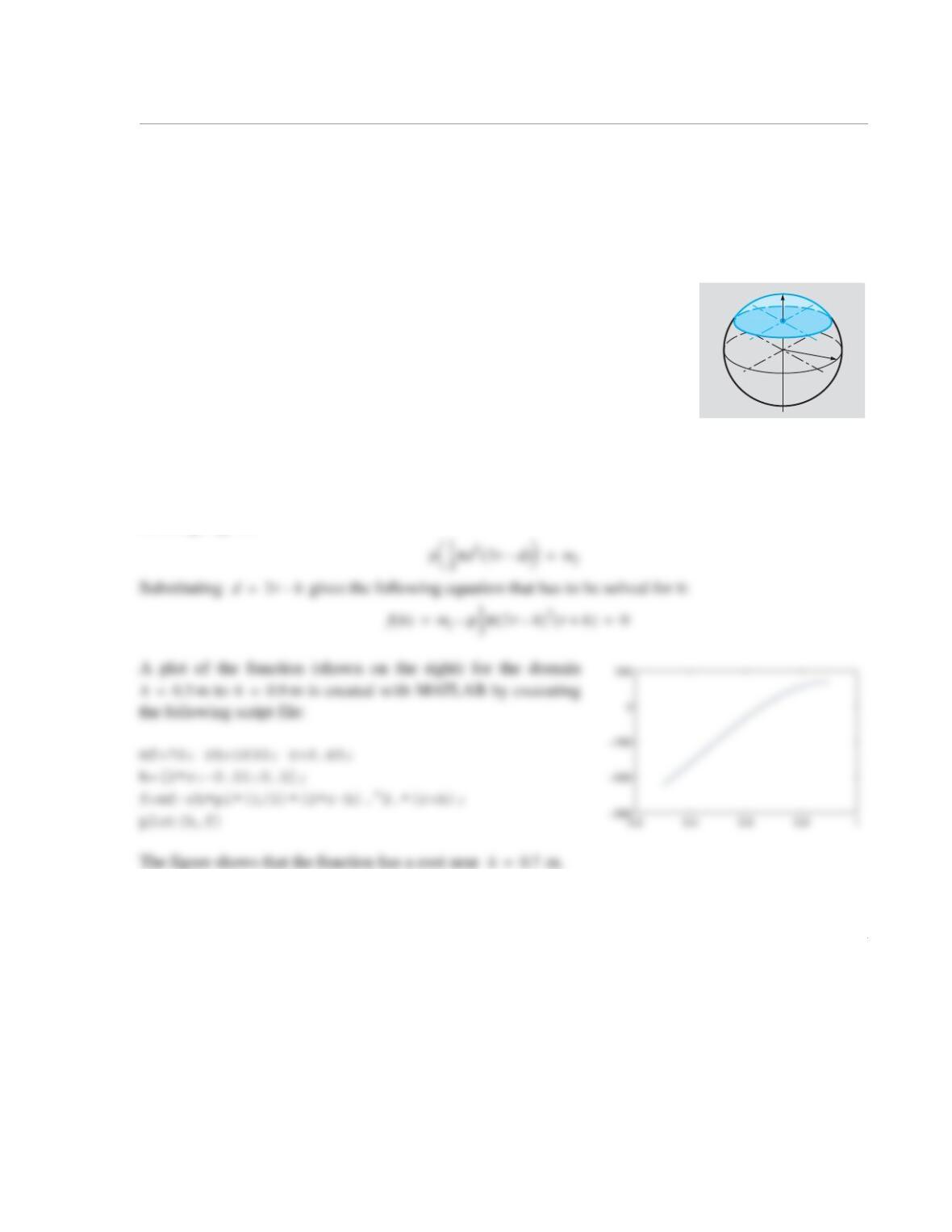
3.33 According to Archimedes’ principle, the buoyancy force acting on an object that is partially

immersed in a fluid is equal to the weight that is displaced by the portion of the object that is submerged.

A spherical float with a mass of kg and a diameter of 90 cm is placed in the ocean (density of

sea water is approximately kg/m3. The height, h, of the portion of the float that is above water

can be determined by solving an equation that equates the mass of the float to the mass of the water that is

displaced by the portion of the float that is submerged:

(1.1)

where, for a sphere of radius r, the volume of a cap of depth d is given by:

Write Eq. (3.59) in terms of h and solve for h.

(a) Use the user-defined function NewtonRoot given in Program 3-2. Use

0.0001 for Err, and 0.8 for Xest.

(b) Use MATLAB’s built-in fzero function.

Solution

Equating the mass of the float to the mass of the water that is displaced by the portion of the float that is

submerged gives:

mf70=

ρ1030=

r

d

ρVcap mf

=

Vcap

1

3

—–πd23rd–()=

2

(a) Solution with Newton method requires also the derivative which is: . To

To use the user-defined function NewtonRoot, the following user-defined functions for and

are written:

function f=HW3_33Fun(h)

The user-defined function NewtonRoot is used in the Command Window:

>> Xs = NewtonRoot(@HW3_33Fun,@HW3_33FunD,0.8,0.0001,10)

Xs =

0.6580

f‘h()

f‘h() ρπ2rh–()h=

fh()

f‘h()

1

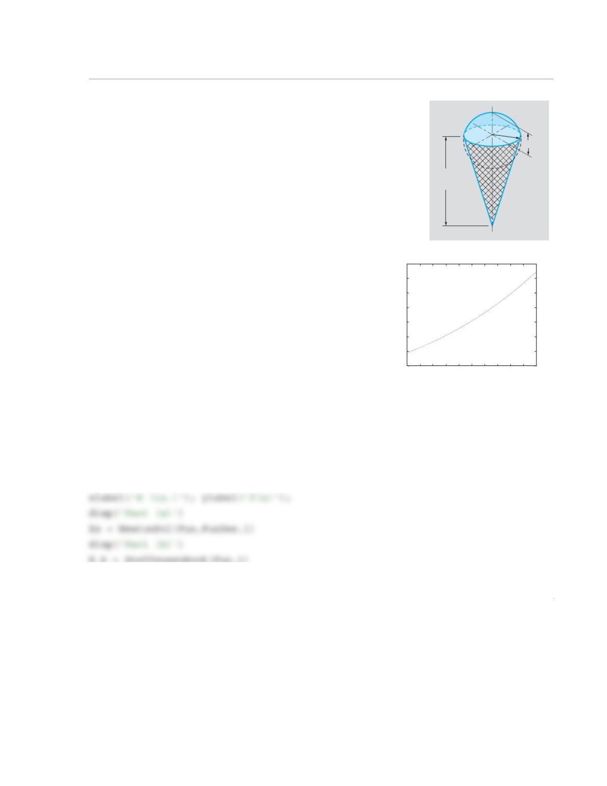
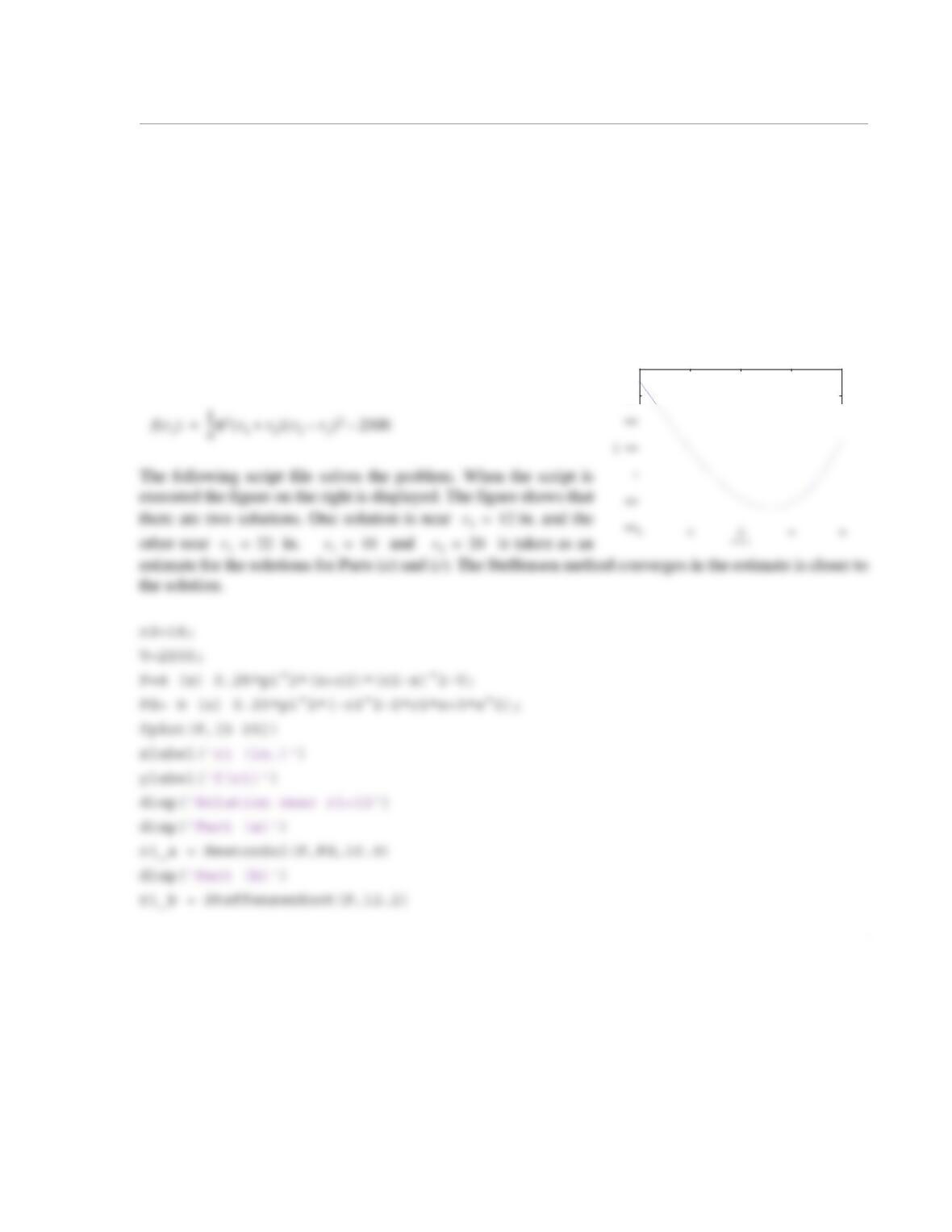
3.34 An ice cream drum is made of a waffle cone filled with ice cream

such that the ice cream above the cone forms a spherical cap. The volume

of the ice cream is given by:

Determine H if U.S. pint (1 U.S pint = 28.875 in3), in.,

in.

(a) Use the user-defined function

NewtonSol

given in Problem 3.22.

(b) Use the user-defined function SteffensenRoot from Problem

3.24.

(c) Use MATLAB’s built-in fzero function.

Solution

The solution is the zero of the function:

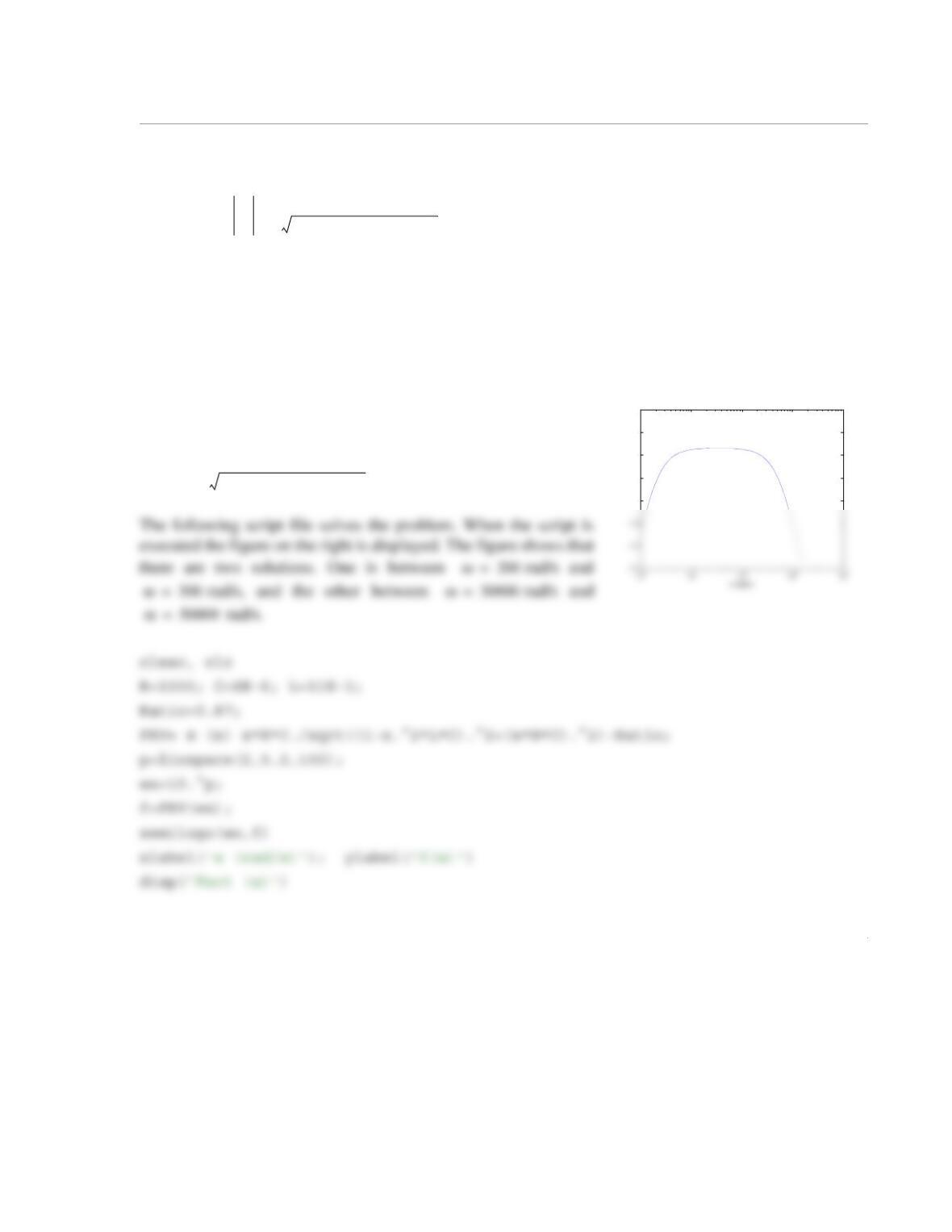
The following script file solves the problem. When the script is

executed the figure on the right is displayed. The figure shows that

the solution is between in. and in. is taken

as an estimate for the solution.

clear, clc

h=4; r=1.1;

V=28.875/3;

Fun=@ (x) pi*(r^2*h/3+x*r^2/2+x^3/6)-V;

FunDer=@ (x) pi*(r^2/2+3*x^2/6);

fplot(Fun,[1 2])

h

H

r

Vπr2h

3

——-–r2H

2

——––H3

6

—––

++





=

V13⁄=

h4=

r1.1=

11.1 1.2 1.3 1.4 1.5 1.6 1.7 1.8 1.9 2

-3

-2

-1

0

1

2

3

4

H (in.)

f(x)

fH() π

r2h

3

——-–r2H

2

——––H3

6

—––

++





28.875

3

—————–

–=

H1=

H2=

H1=

2

disp(‘Part (c)’)

H_c=fzero(Fun,1)

When the script file is executed the following solution is displayed in the Command Window:

1

3.35 A bandpass filter passes signals with frequencies that are within a certain range. In this filter the

ratio of the magnitudes of the voltages is given by

where is the frequency of the input signal. Given Ω, mH, and µF, determine the

frequency range that corresponds to .

(a) Use the user-defined function BisectionRoot that was developed in Problem 3.16.

(b) Use the user-defined function SteffensenRoot from Problem 3.24.

(c) Use MATLAB’s built-in function fzero.

Solution

The solution is the zero of the function:

RV Vo

Vi

—– ωRC

1ω2LC–()

2ωRC()

2

+

————————————-——————-—-–

==

ω

R1000=

L11=

C8=

RV 0.87≥

-0.1

0

0.1

0.2

0.3

f(w)

fω() ωRC

1ω2LC–()

2ωRC()

2

+

—————–——————-——————-—––0.87–=

2

wa1 = BisectionRoot(FRV,200,300)

wa2 = BisectionRoot(FRV,30000,60000)

fprintf(‘ The frequency range is between %G6 rad/s and %G6 rad/s\n’,wa1,wa2)

When the script file is executed the following results are displayed in the Command Window.

Part (a)

wa1 =

219.6288

1

3.36 Determining the value of is the same as calculating the root of the function .

Determine the root, to accuracy of five decimal points, with the bisection method. Use the user-defined

function BisectionRoot from problem 3.16. Compare the result with the value calculated with a calcu-

lator.

Solution

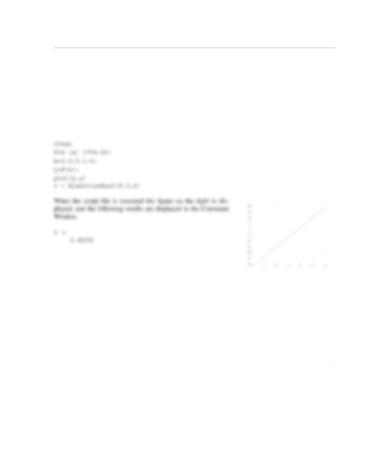
The problem is solved in the following script. It first make a plot of as a function of x for .

The plot shows that the solution is between 3 and 5. Then the function is solved.

65 17⁄

fx() 17x65–=

fx()

0.5 x6≤≤

fx() 0=

1

3.37 The power output of a solar cell varies with the voltage it puts out. The voltage at which the out-

put power is maximum is given by the equation:

where is the open circuit voltage, T is the temperature in Kelvin, C is the charge on

an electron, and J/k is Boltzmann’s constant. For V and room temperature

( K), determine the voltage at which the power output of the solar cell is a maximum.

(a) Write a program in a script file that uses the fixed-point iteration method to find the root. For starting

point, use V. To terminate the iterations, use Eq. (3.18) with .

(b) Use MATLAB’s fzero built-in function.

Solution

To estimate the solution, the function is plotted for the domain

to . The following user-defined function calculates for a given value of .

Vmp

eqVmp kB

⁄T()

1qVmp

kBT

———––

+





eqVOC kB

⁄T()

=

VOC

q1.6022 10 19–

×=

kB1.3806 10 23–

×=

VOC 0.5=

T297=

Vmp

Vmp 0.5=

ε0.001=

fV

mp

()eqVmp kB

⁄T()

1qVmp

kBT

———––

+





eqVOC kB

⁄T()

–=

Vmp 0.1=

Vmp 0.45=

fV

mp

()

Vmp

Vmp 0.4=

Vmp 0.45=

2

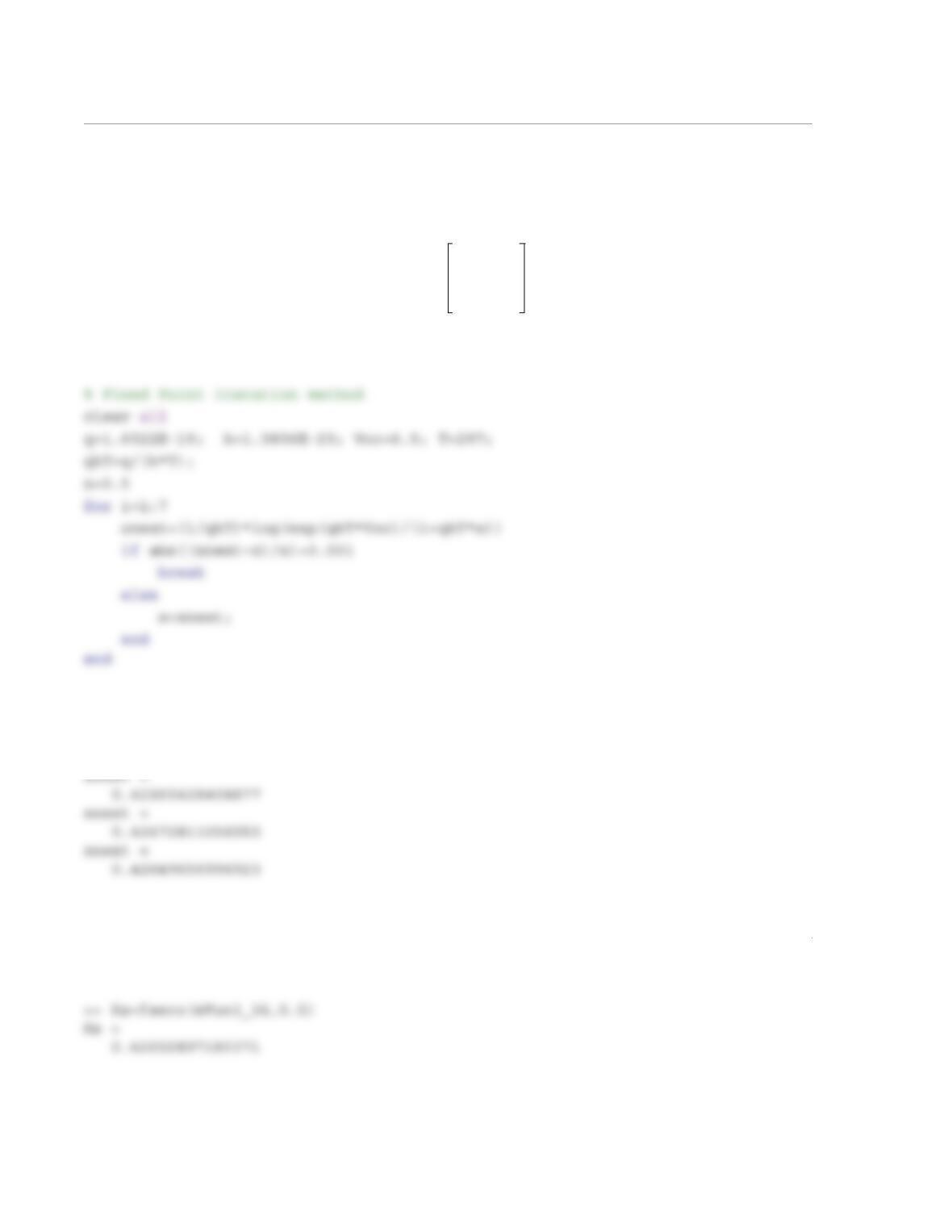
(a) To use the fixed-point iteration method the equation is solved for

:

This iteration function is used in the following MATLAB program (Script file). For starting point the value

V is used. The iterations are terminated by using Eq. (3.18) with .

When the program is executed, the display in the Command Window is:

x =

0.50000000000000

eqVmp kB

⁄T()

1qVmp

kBT

———––

+





eqVOC kB

⁄T()

=

Vmp

kT

q

—––eqVOC kB

⁄T()

1qVmp

kBT

———––

+

—————-——––

ln=

Vmp 0.5=

ε0.001=

The iterations stop after the third iteration.

(b) MATLAB’s built-in function fzero is used in the Command window to find the root.

1

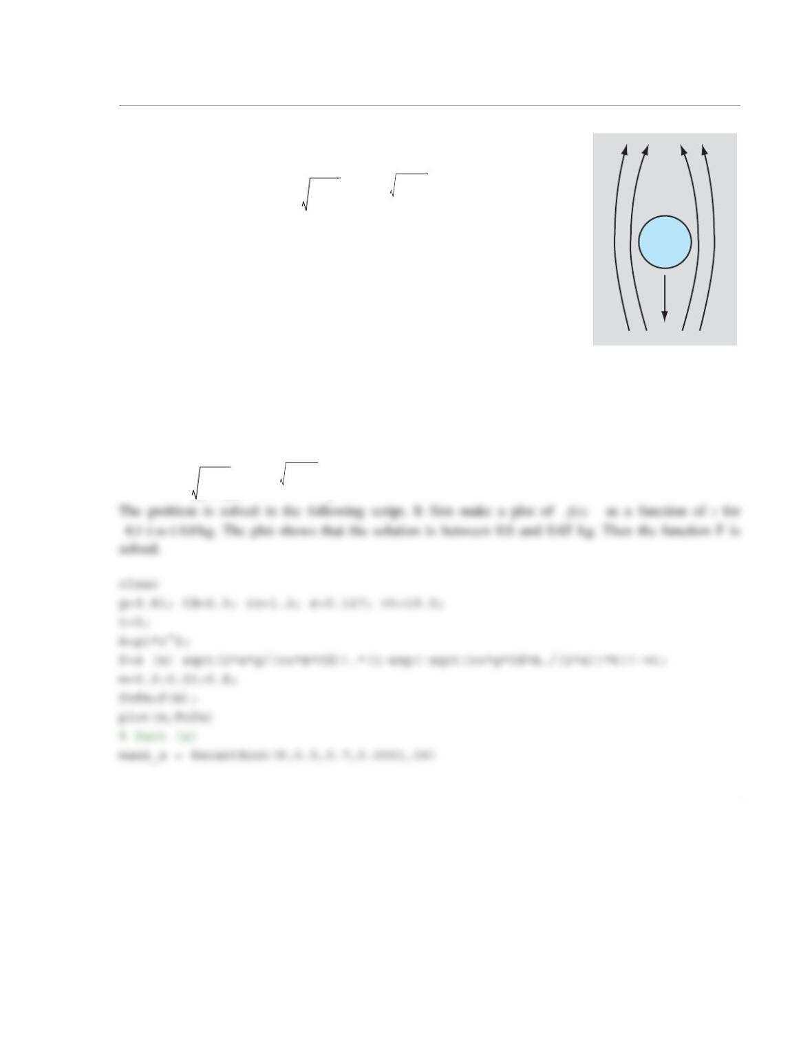
3.38 The volume V of a torus-shaped water tube is given by:

where and are the inside and outside radii, respectively, as shown in the figure. Determine if

in2 and in.

(a) Use the user-defined function

NewtonSol

given in Problem 3.22.

(b) Use the user-defined function SteffensenRoot from Problem 3.24.

(c) Use MATLAB’s built-in fzero function.

Solution

The solution is the zero of the function:

V1

4

—–π2r1r2

+()r2r1

–()

2

=

r1

r2

r1

V2500=

r218=

6000

8000

2

disp(‘Solution near r1=22’)

r1_a = NewtonSol(F,Fd,20.0)

disp(‘Part (b)’)

r1_b = SteffensenRoot(F,23)

disp(‘Part (c)’)

r1_c=fzero(F,20)

When the script file is executed the following results are displayed in the Command Window:

Solution near r1=12

Part (a)

r1_a =

12.2086

1

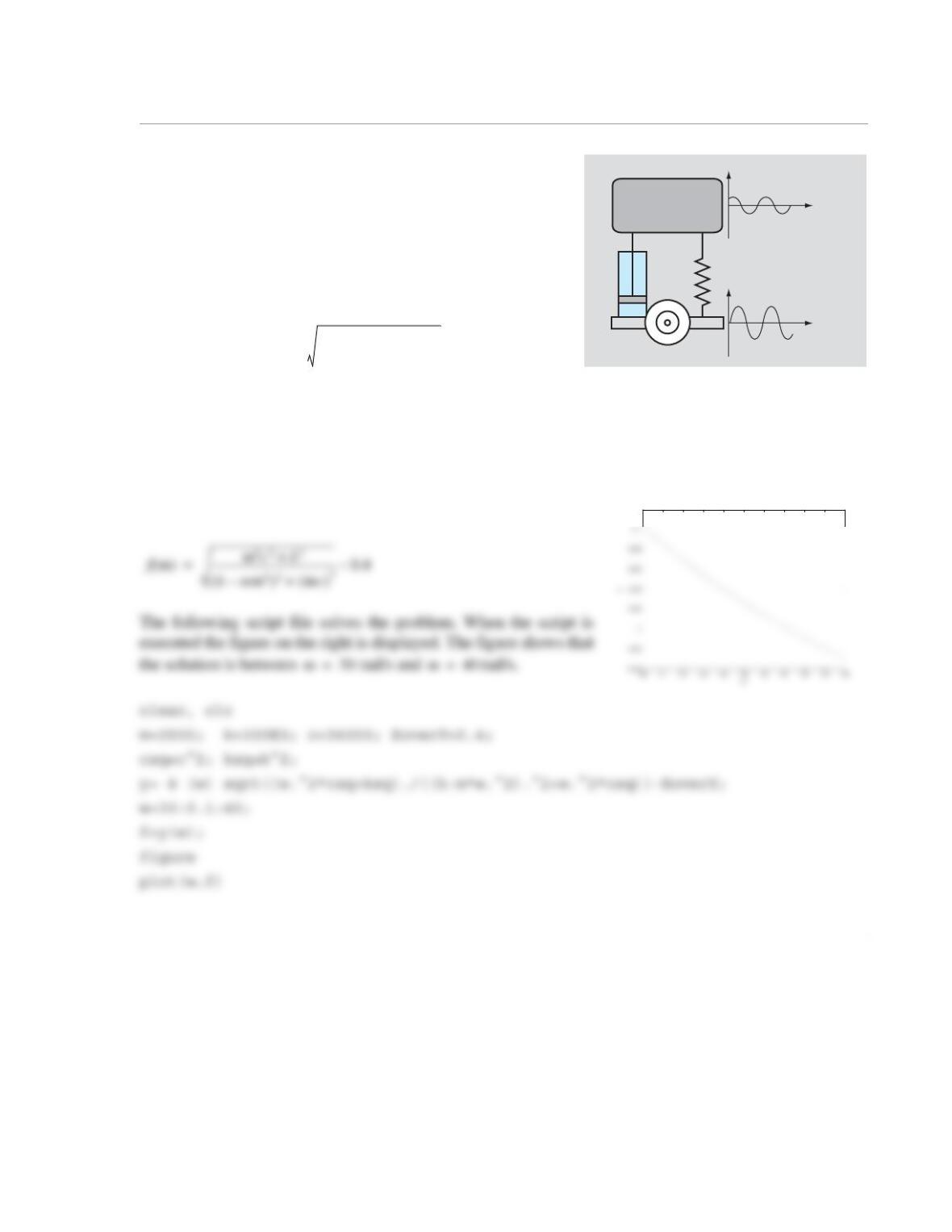
3.39 A simplified model of the suspension of a car consists of

a mass, m, a spring with stiffness, k, and a dashpot with damp-

ing coefficient, c, as shown in the figure. A bumpy road can be

modeled by a sinusoidal up-and-down motion of the wheel

. From the solution of the equation of motion for

this model, the steady-state up-and-down motion of the car

(mass) is given by . The ratio between ampli-

tude X and amplitude Y is given by:

Assuming kg, kN/m, and N-s/m, determine the frequency ω for which

. Rewrite the equation such that it is in the form of a polynomial in and solve.

(a) Use the user-defined function BisectionRoot that was developed in Problem 3.16.

(b) Use MATLAB’s built-in fzero function.

Solution

The solution is the zero of the function:

m

k

c

t

y

x

xX ωtφ–()sin=

yY ωt()sin=

xX ωtφ–()sin=

X

Y

—– ω2c2k2

+

kmω2

–()

2ωc()

2

+

—————–——————-———-–=

m2500=

k300=

c36 103

×=

XY⁄0.4=

ω

0.12

2

xlabel(‘w’); ylabel(‘f’)

disp(‘Part (a)’)

w_a = BisectionRoot(y,30,40)

disp(‘Part (b)’)

w_b=fzero(y,30)

When the script is executed, the following results are displayed in the Command Window:

1

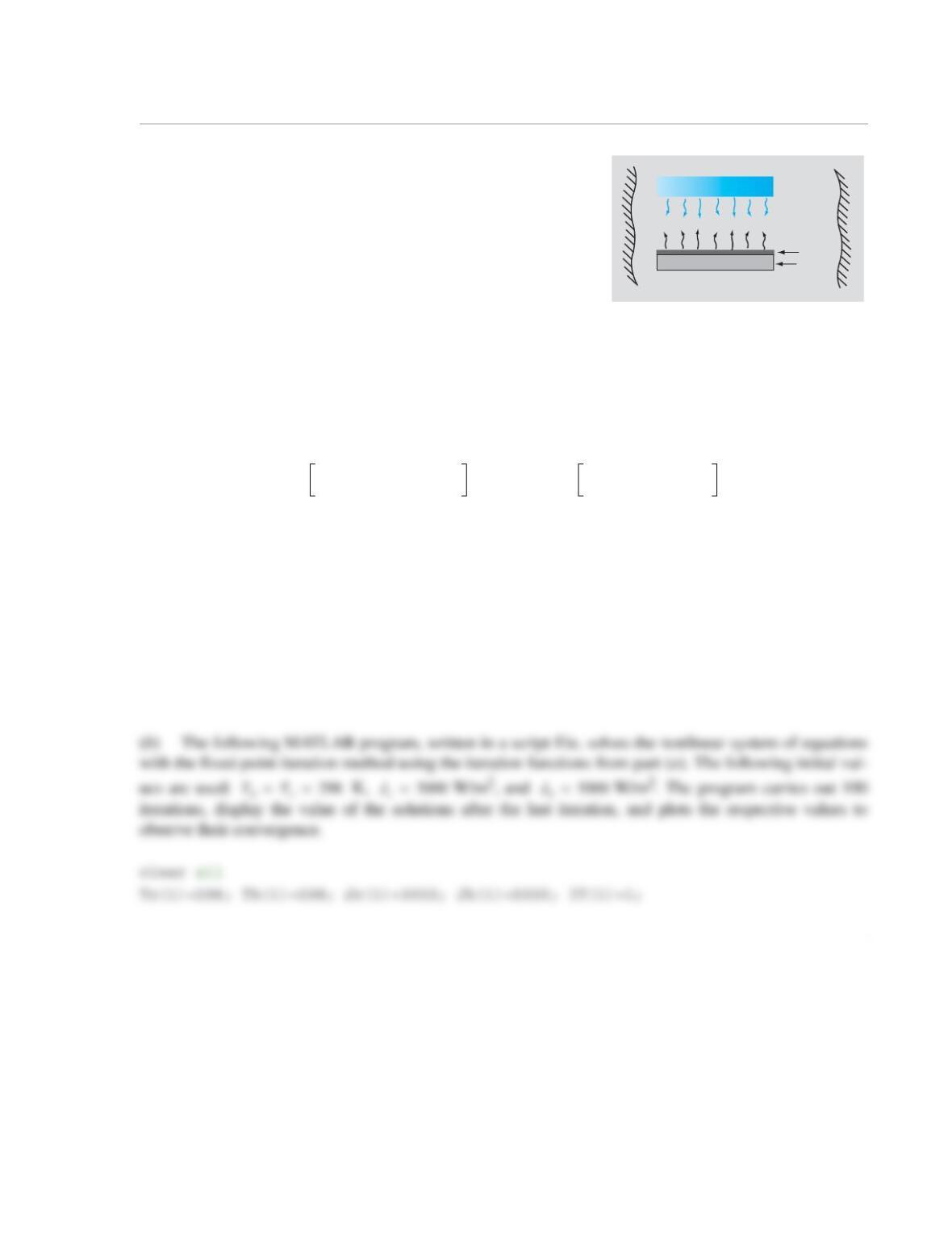
3.40 A coating on the panel surface is cured by radiant energy

from a heater. The temperature of the coating is determined by

radiative and convective heat transfer processes. If the radiation is

treated as diffuse and gray, the following nonlinear system of

simultaneous equations determine the unknowns , , , :

where and are the radiosities of the heater and coating surfaces, respectively, and and are the

respective temperatures.

(a) Show that the following iteration function can be used for solving the nonlinear system of equations

with the fixed-point iteration method:

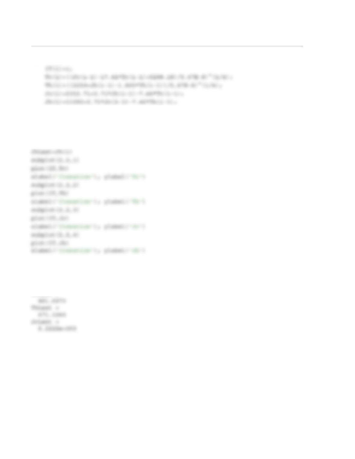
(b) Solve the nonlinear system of equations with the fixed-point iteration method using the iteration func-

tions from part (a). Use the following initial values: K, W/m2, and

W/m2. Carry out 100 iterations, and plot the respective values to observe their convergence.

The final answers should be: K, W/m2, K, W/m2.

Solution

(a) The iteration functions are derived by solving the first equation for , the second equation for ,

the third equation for , and the fourth equation for .

coating

panel

Ambient at

298 K

Jh

Th

Jc

Tc

5.67 10 8–

×Tc

417.41TcJc

–+ 5188.18=

Jc0.71Jh

–7.46Tc

+ 2352.71=

5.67 10 8–

×Th

41.865ThJh

–+ 2250=

Jh0.71Jc

–7.46Th

+ 11093=

Jh

Jc

Th

Tc

Jc17.41Tc

– 5188.18+

5.67 10 8–

×

——————-——————-—————-–

14⁄

=

Jc2352.71 0.71Jh7.46Tc

–+=

Th

2250 Jh1.865Th

–+

5.67 10 8–

×

——————-—————————–

14⁄

=

Jh11093 0.71Jc7.46Th

–+=

ThTc298==

Jc3000=

Jh5000=

Tc481=

Jc6222=

Th671=

Jh10504=

Tc

Jc

Th

Jh

ThTc298==

Jc3000=

Jh5000=

2

for i=2:100

end

i

TcLast=Tc(i)

ThLast=Th(i)

JcLast=Jc(i)

When the program is executed, the following is displayed in the Command Window.

i =

100

TcLast =

3

JhLast =

1.0504e+004

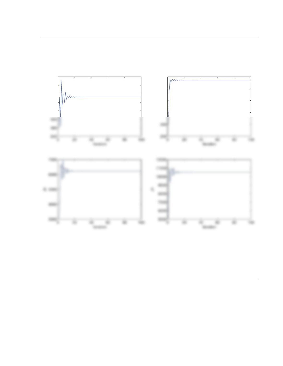
The following figure is displayed in the Figure Window.

400

450

500

550

600

Tc

400

500

600

700

Th

1

3.41 If a basketball is dropped down from a helicopter, its velocity as a

function of time can be modeled by the equation:

where m/s2 is the gravitation of the Earth, is the drag

coefficient, kg/m3 is the density of air, is the mass of the basket-

ball in kg, and is the projected area of the ball ( m is the

radius). Note that initially the velocity increases rapidly, but then due to the

resistance of the air, the velocity increases more gradually. Eventually the

velocity approaches a limit that is called the terminal velocity. Determine

the mass of the ball if at s the velocity of the ball was measured to be

19.5 m/s.

(a) Use the user-defined function SecantRoot given in Program 3-3. Use 0.0001 for Err.

(b) MATLAB’s built-in fzero function.

Solution

The solution is obtained by finding the root, of the function:

v

vt()

vt() 2mg

ρACd

————-–1e

ρgCdA

2m

———-——- t–

–







=

g9.81=

Cd0.5=

ρ1.2=

m

Aπr2

=

r0.117=

t5=

Fm() 2mg

ρACd

————-–1e

ρgCdA

2m

———-——- t–

–







vt()–=

2

% Part (b)

mass_b=fzero(F,0.5)

When the script file is executed the figure on the right is dis-

played, and the following results are displayed in the Command

Window.

0

1

2