3
(c) Using MATLAB built-in functions to solve the ODE.
The ODE is transforming into a system of two first-order ODEs:
11.5 22.5 33.5
500
600
r (cm)
dT
dr
—–– w=
dw
dr
——–1–
r
—––w500–
r
———––
–=
4
function res = bcfunHW11_21_3ed(Ta,Tb)
BCa = 600; BCb = 25;
res = [Ta(1) – BCa
Tb(1) – BCb];
The program in the following script file solves the problem:
% Solution of HW11_21c_3ed (Script file)
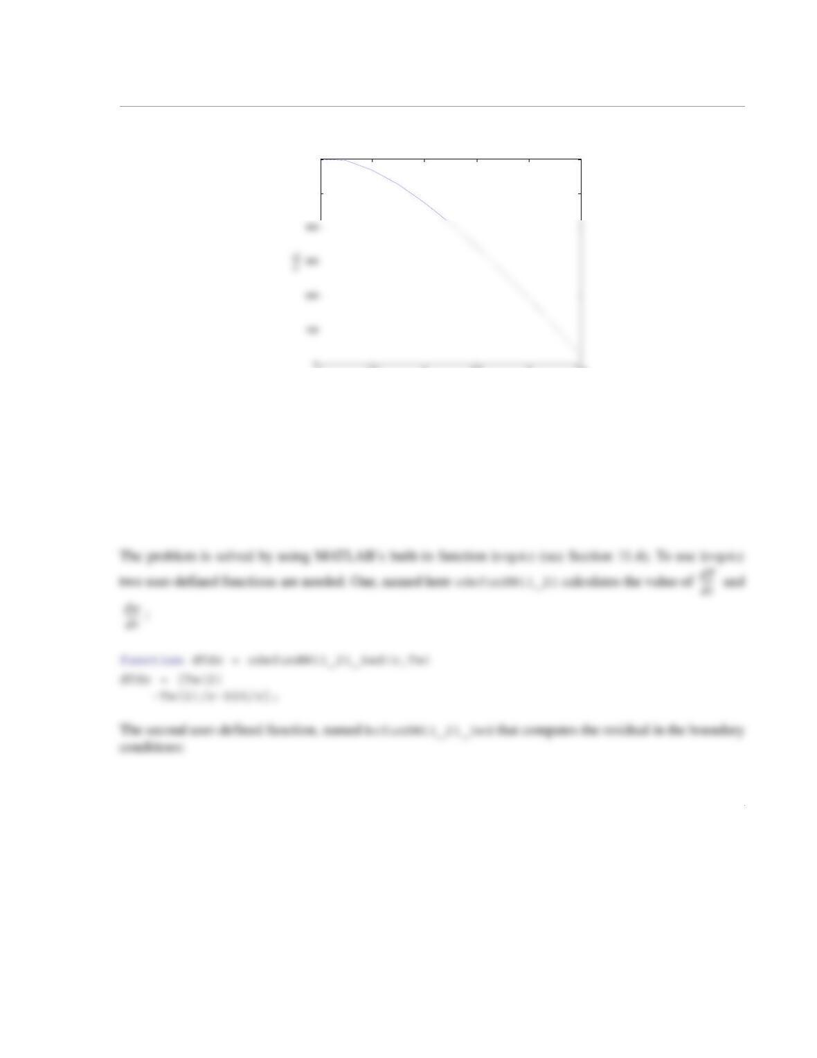
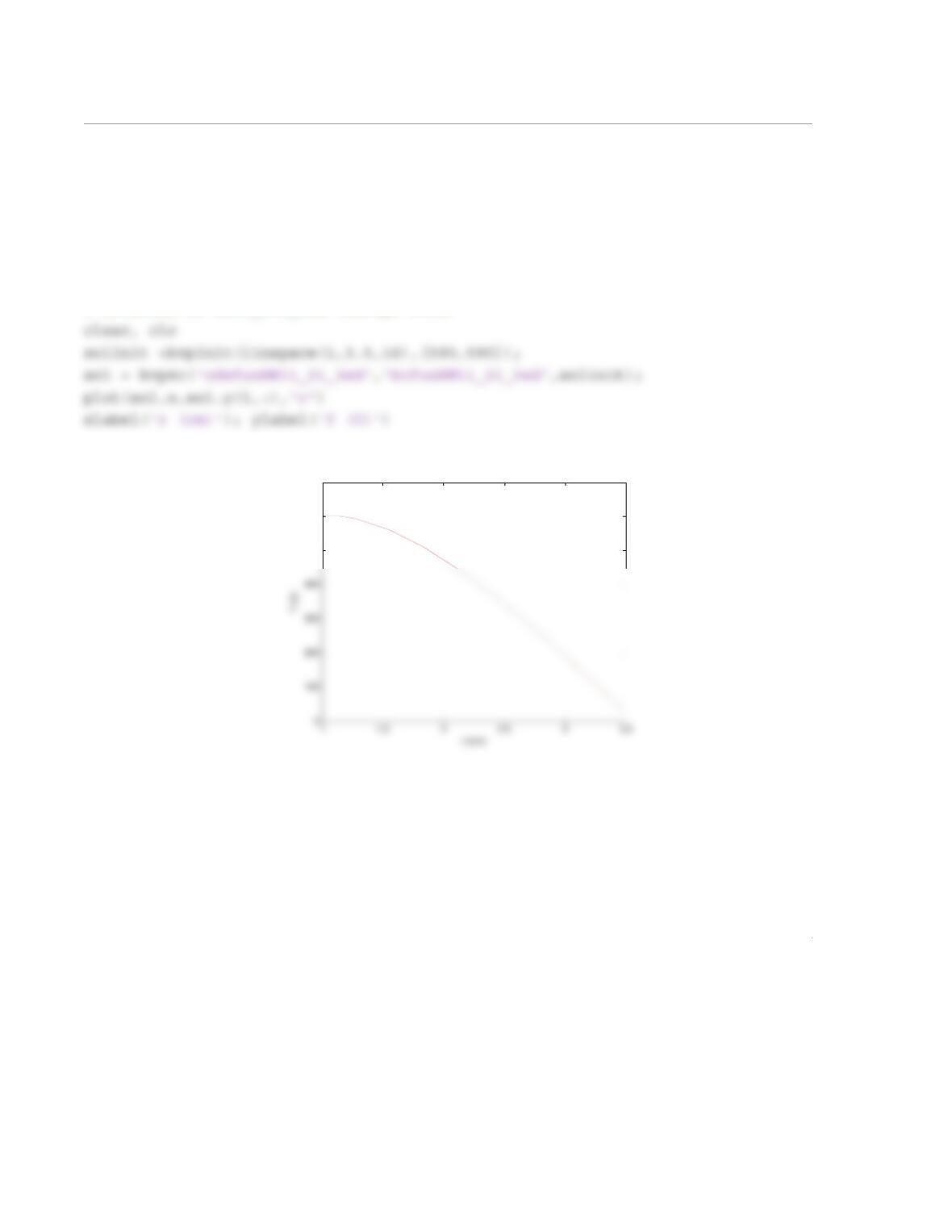
When the script file is executed, the following figure is displayed in the Figure Window:
500
600
700
1
11.22 Solve Problem 11.21 subject to the boundary conditions and
.
Solution
Using MATLAB built-in functions to solve the ODE.
The ODE is transforming into a system of two first-order ODEs:
T1() 600=
dT
dr
—––
r3.5=
0.1 T3.5()25–()=
dT
dr
—–– w=
dw
dr
——–1–
r
—––w500–
r
———––
–=
2
sol = bvp4c(‘odefunHW11_22_3ed’,‘bcfunHW11_22_3ed’,solinit);
plot(sol.x,sol.y(1,:),‘r’)
xlabel(‘r (cm)’); ylabel(‘T (C)’)
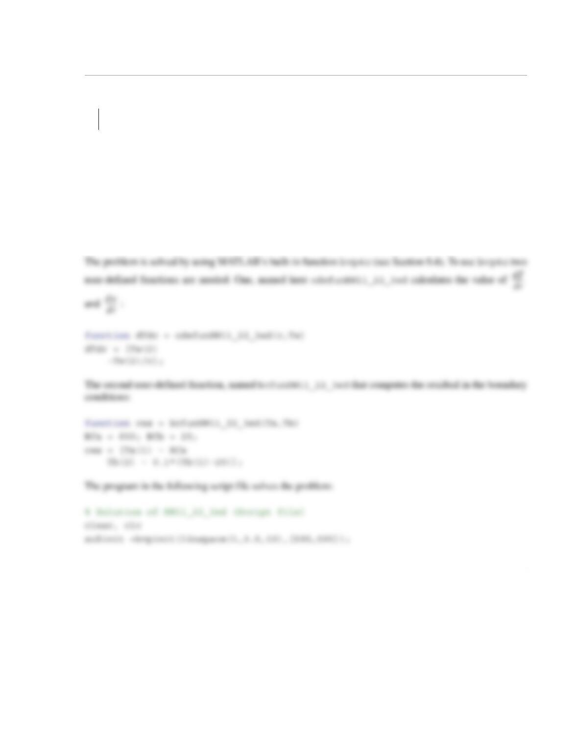
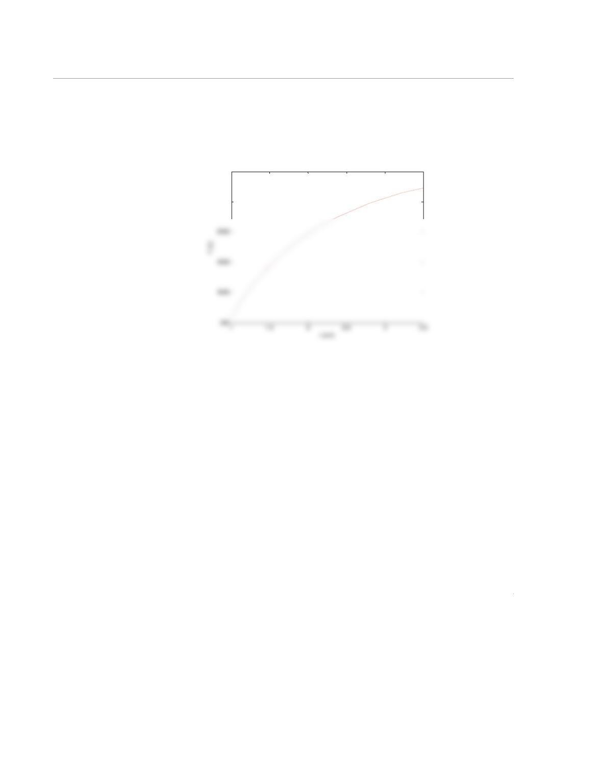
When the script file is executed, the following figure is displayed in the Figure Window:
2500
3000
1
11.23 The temperature distribution in a straight fin, , with a trian-
gular profile is given by the solution of the equation:
where K is the ambient temperature, x is the coordinate mea-
sured along the fin, W/m/K is the thermal conductivity of alu-
minum, W/m2/K is the convective heat transfer coefficient,
m is the length of the fin, m is its width, and
m is the height of the base. The boundary conditions are
K, and .
Find and plot the temperature distribution, , along the fin. Write a program in a script file that solves
the problem with the shooting method. Note that a derivative boundary condition is prescribed at .
Use the three-point backward difference formula to calculate the value of the derivative from the numerical
solution at . Compare the numerical solution with the prescribed boundary condition and use the
bisection method to calculate the new estimate for the slope at . Iterate until the true relative error at
is smaller than 0.01. Important note: The point is a singular point of the ODE. Therefore,
the problem cannot be solved as specified. An approximate solution can, however, be obtained by using
m for the length of the fin.
Solution
First, the second order ODE is written as a system of two first order ODEs:
x
L
W
b
Tx()
d2T
dx2
——–– 1
Lx–()
—————– dT
dx
—––
–2hLW bL bx–+()TT
∞
–()
kbW L x–()
—————-———————————-—————–
–0=
T∞300=
k237=
h15=
L0.01=
W0.1=
b0.01=
Tx 0=()1073=
dT
dx
—––
xL=
0=
Tx()
xL=
xL=
x0=
xL=
xL=
L0.00999999=
dT
dx
—–– w=
dT
dx
—––
xL=
0=
xL=
2
ODEs with the user-defined function Sys2ODEsRK4 that was written in Example 10-8. The values of the
two first-order ODEs, and , are calculated in two user-defined functions named ODE1 and ODE2
(they are listed following the script file).
h=(b-a)/n;
% Calculate the first two solutions.
[x TH zL] = Sys2ODEsRK4(@ODE1,@ODE2,a,b,h,Ta,WH);
[x TL zH] = Sys2ODEsRK4(@ODE1,@ODE2,a,b,h,Ta,WL);
iLast=length(x);
% Calculate dT/dx at x=L (using the three-point backward difference formula)
% for the first two solutions.
DTH=(TH(iLast-2)-4*TH(iLast-1)+3*TH(iLast))/(2*h);
DTL=(TL(iLast-2)-4*TL(iLast-1)+3*TL(iLast))/(2*h);
dT
dx
—––
dw
dx
——–
3
DTi=(Ti(iLast-2)-4*Ti(iLast-1)+3*Ti(iLast))/(2*h);
E = DTi – DTb;
if abs(E) < tol
break
fprintf(‘Solution was not obtained in %i iterations.\n’,imax)
end
end
plot(x,Ti)
xlabel(‘x (m)’), ylabel(‘T (K)’)
The two user-defined functions ODE1 and ODE2 are:
function dTdx=ODE1(x,T,w)
dTdx=w;
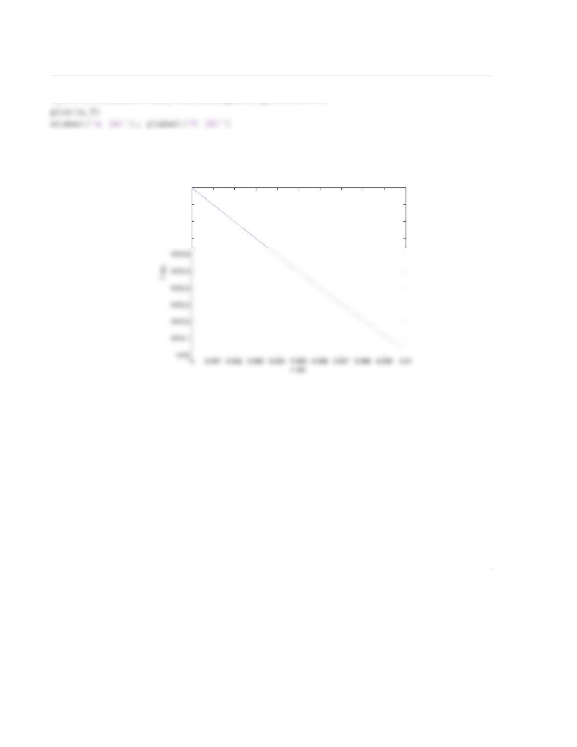
When the script file is executed the following plot (solution) is displayed:
1072.7
1072.8
1072.9
1073
1
11.24 Solve Problem 11.23 using the finite difference method with 100 subintervals. Use second-order
accurate central differences for all the derivatives in the ODE, and use appropriate one-sided differences
for the boundary condition. As explained in Problem 11.23, use m for the length of the fin.
Solution
The problem is solved by using the user-defined function BVP2ndDriv that was written in Problem
11.17. The equation that is being solved is:
In order to solve the problem, the following three user-defined functions that calculate , and
are written:
function px=pOFx(x)
L=0.00999999;
px=-1/(L-x);
The following program (script file) solves the problem:
% Solution of Problem 11.24
clear
a=0; b=0.00999999; n=100; Ta=1073; Db=0;
L0.00999999=
d2T
——–– 1
Lx–()
—————– dT
dx
—––
–2hLW bL bx–+()TT
∞
–()
kbW L x–()
—————————————————-————-–
–0=
px()
qx()
rx()
2
[x,T]=BVP2ndDeriv(a,b,Ta,Db,n,@pOFx,@qOFx,@rOFx);
The listing of the user-defined function BVP2ndDeriv is given in the solution of Problem 11.17.
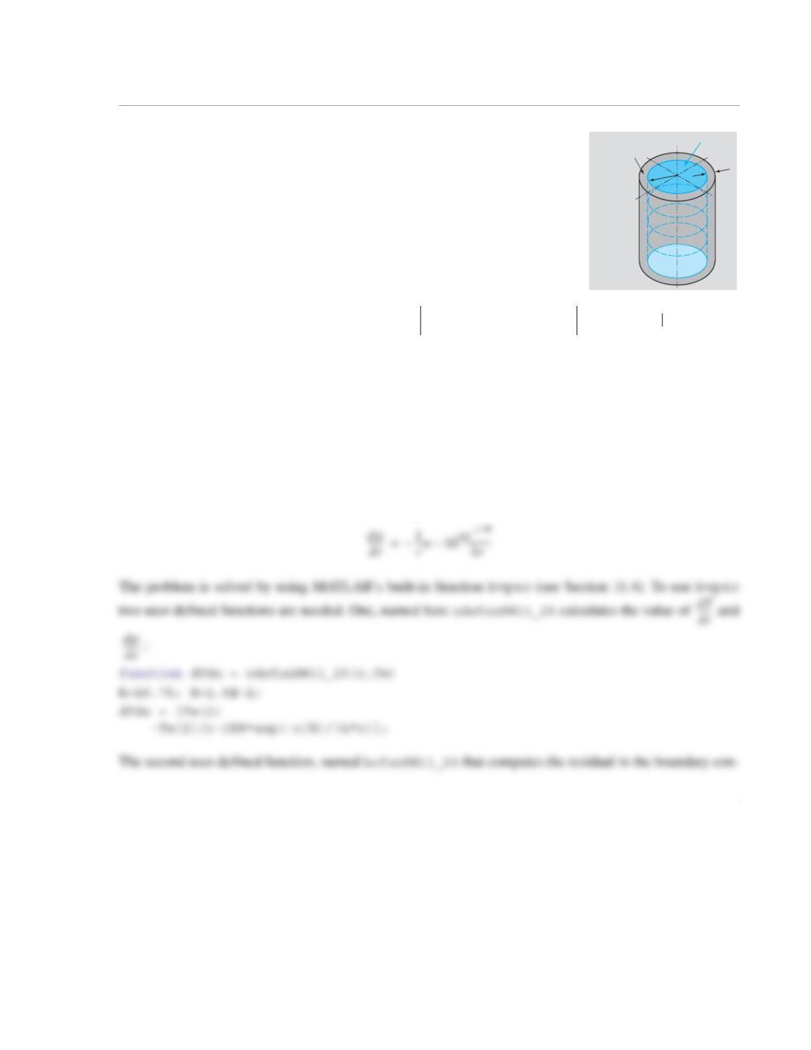
When the program is executed, the following plot (solution is displayed:
1072.7
1072.8
1072.9
1073
1
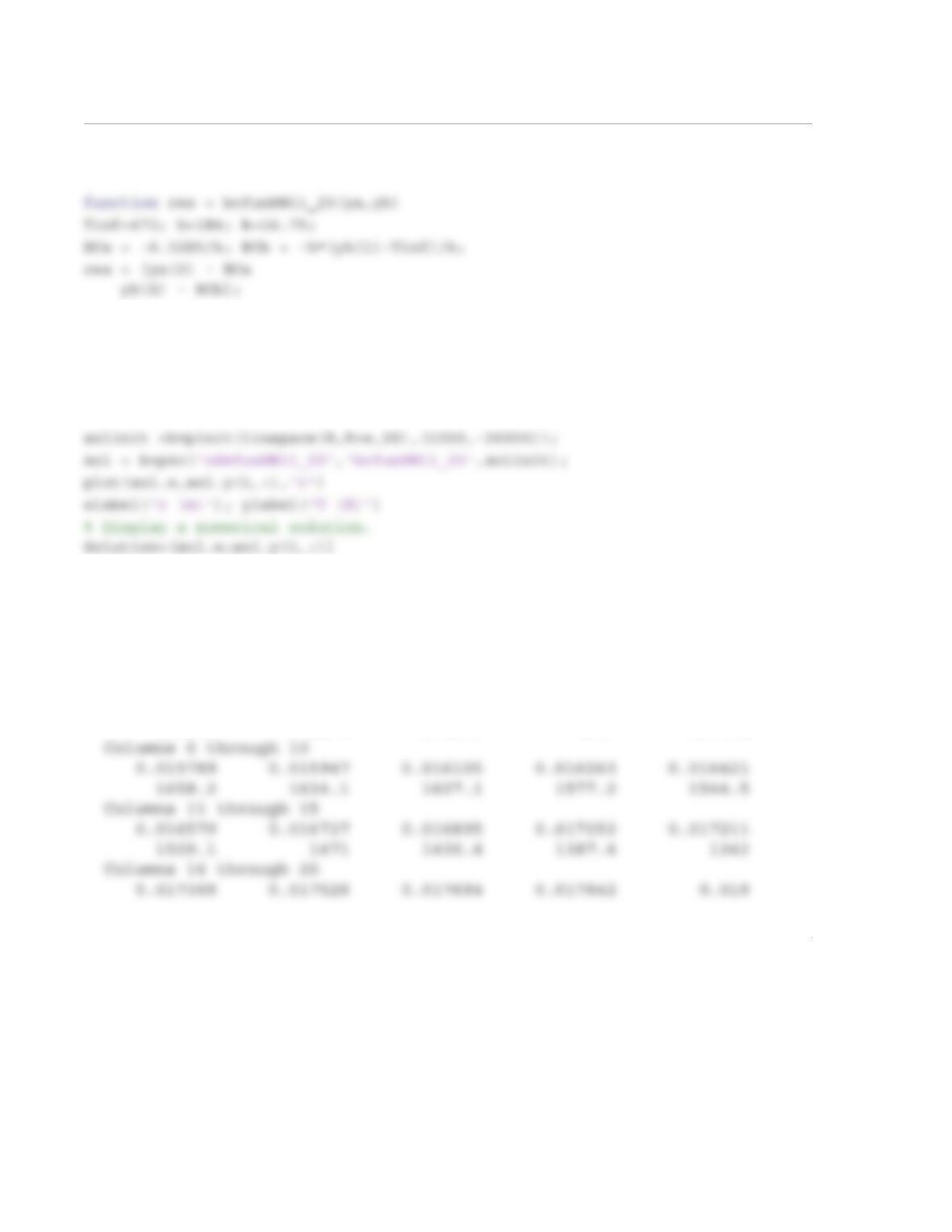
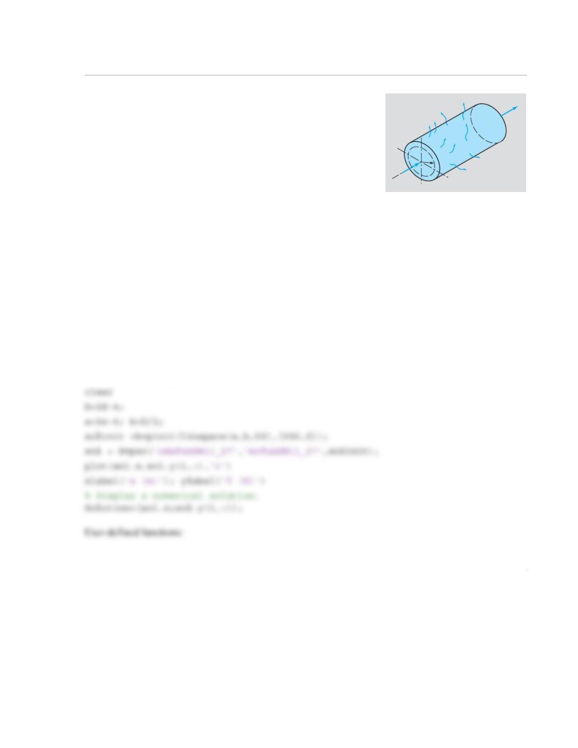
11.25 The fuel rod of a nuclear reactor is a cylindrical structure with the fuel
retained inside a cladding, as shown in the figure. The fuel causes heat to be
generated by nuclear reactions within the cylinder as well as in the cladding.
The outer surface of the cladding is cooled by flowing water at K
with a heat transfer coefficient of W/m2/K. The thermal conductivity
of the cladding material is W/m/K. The dimensions of the fuel rod
are m, and m. The temperature distribution in
the cladding is determined by the solution of the following boundary value
problem:
, for , with and
Use MATLAB’s built-in function bvp4c to solve the boundary value problem. Plot the temperature distri-
bution in the cladding as a function of r.
Solution
The ODE can be written in the form:
The ODE is transforming into a system of two first-order ODEs:
R
w
Cladding
Fuel
T∞473=
h104
=
k16.75=
R1.5 10 2–
×=
w3.0 10 3–
×=
1
r
—–d
dr
—-– rkdT
dr
—––
10– 8erR⁄–
r
———––
=
RrRw+≤≤
dT
dr
—––
rR=
6.32 105
×
k
————————–
–=
dT
dr
—––
rRw+=
h
k
—–TrRw+= T∞
–()–=
d2T
dr2
——––1
r
—–dT
dr
—––
–10
8erR⁄–
kr
———––
–=
dT
dr
—–– w=
dx
2
ditions:
The program in the following script file solves the problem:
% Solution HW11_25 (Script file)
clear
R=1.5E-2; w=3E-3;
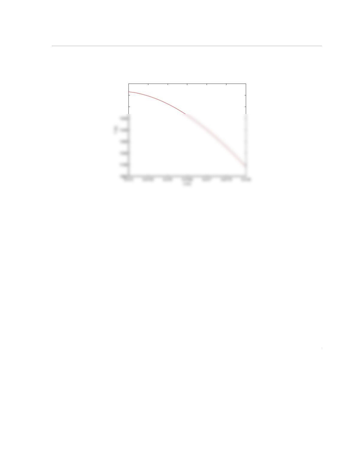
When the script file is executed, the following numerical solution is displayed in the Command Window,
and the following plot of the solution is displayed in the Figure Window:
>> format short g
Solution =
Columns 1 through 5
0.015 0.015158 0.015316 0.015474 0.015632
1730.6 1722.8 1711.6 1697 1679.2
3
1294.2 1244.2 1192 1137.7 1081.4
1600
1700
1800
1
11.27 The radial distribution of temperature in a current-carrying bare
wire is described by:
where T is the temperature in K, r is the radial coordinate in m,
W/m/K is the thermal conductivity, A is the current,
-m is the electrical resistivity, and m is
the wire diameter. Use MATLAB’s built-in function bvp4c to solve the equation for . Solve twice for
the following boundary conditions:
(a) At m, and at , K.
(b) At m, and at , , where W/m2 is the con-
vection heat transfer coefficient and K is the ambient temperature.
Important note: is a singular point and must therefore be replaced with a small, non-zero value. As
initial guesses, use K and , and use 50 subintervals.
Solution
(a) The following script solves this problem:
% Solution HW11_27
T
8
Ir
I
k
r
— d
dr
—-– rdT
dr
—––
I2ρe
1
4
—–πD2
2
———————–
–=
k72=
I0.5=
ρe32 10 8–
×=
Ω
D110
4–
×=
Tr()
r10 6–
=
dT
dr
—–– 0=
rD2⁄=
T300=
r10 6–
=
dT
dr
—–– 0=
rD2⁄=
dT
dr
—–– h
k
—–Tr D 2⁄=()T∞
–()–=
h100=
T∞300=
r0=
T500=
dT
dr
—–– 0=
2
function dTdr = odefunHW11_27(r,Tw)
k=72; h=100; I=0.5;
roe=32E-8; Tinf=300; D=1E-4;
dTdr = [Tw(2)
-Tw(2)/r-I^2*roe/(k*(pi*D^2/4)^2)];
When executed, the program produces the following plot:
300.01
300.015