1
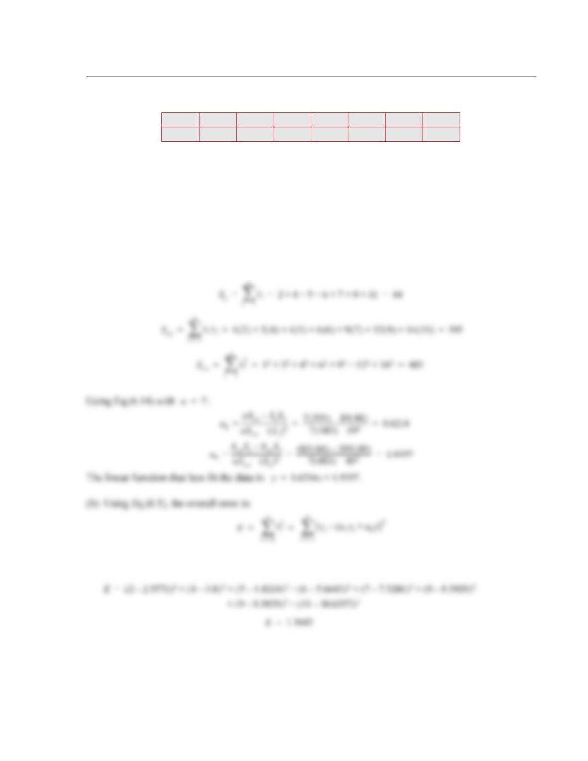
6.1 The following data is given:
(a) Use linear least-squares regression to determine the coefficients m and b in the functi on
that best fit the data.
(b) Use Eq. (6.5) to determine the overall error.
Solution
(a) In the equation , corresponds to and corresponds to in the discussion of Section
6.2.2. Using Eq.(6.13),
x1 3 4 6 9 12 14
y2 4 5 6 7 9 11
ymxb+=
ymxb+=
m
a1
b
a0
Sxxi
i1=
n
134691214+++++ + 49== =
1
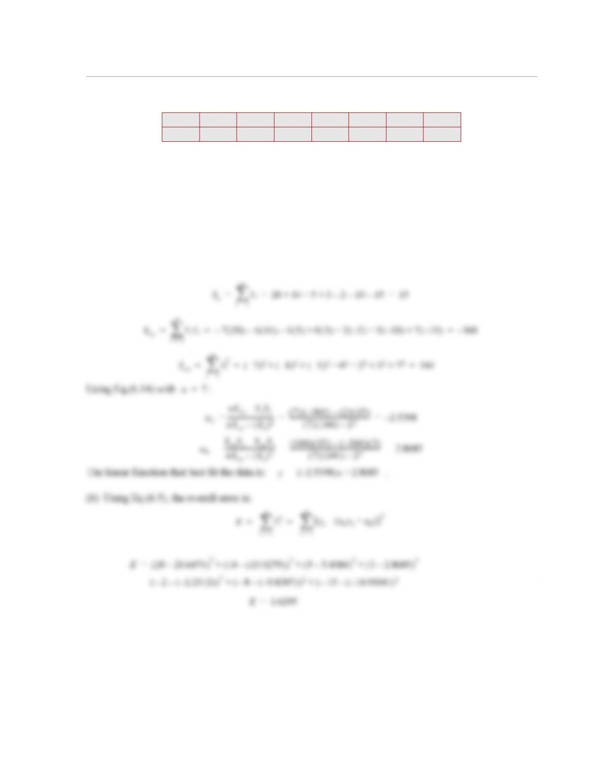
6.2 The following data is given:
(a) Use linear least-squares regression to determine the coefficients m and b in the functi on
that best fit the data.
(b) Use Eq. (6.5) to determine the overall error.
Solution
(a) In the equation , corresponds to and corresponds to in the discussion of Section
6.2.2. Using Eq.(6.13)
x–7 –4 –1 0 2 5 7
y20 14 5 3 –2 –10 –15
ymxb+=
ymxb+=
m
a1
b
a0
Sxxi
i1=
n
7–4–1–0257++++ 2== =
1
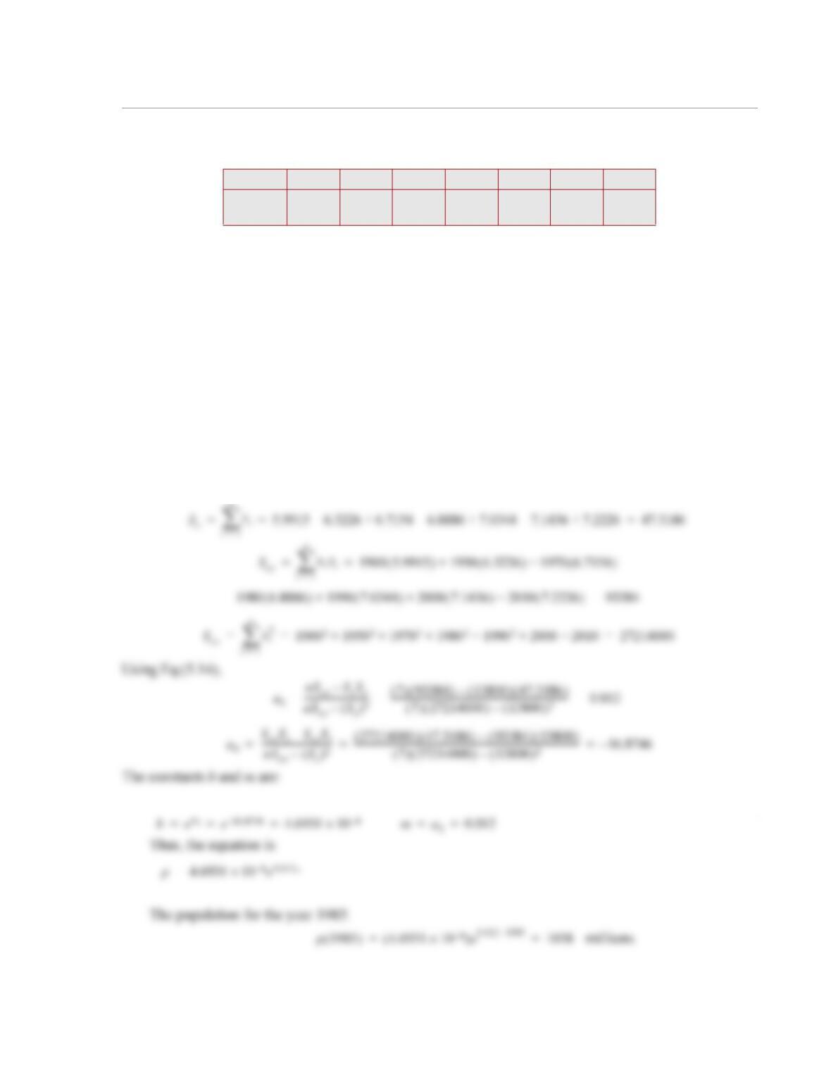
6.3 The following data give the approximate population of Chin a for selected years from 1900 until
2010:
Assume that the population growth can be modeled with an exponential function , where x is the
year and p is the population in millions. Write the equation in a linear form (Section 6.3), and use linear
least-squares regression to determine the constants b and m for which the function best fits the data. Use the
equation to estimate the population in the year 1985.
Solution
For , take the natural logarithm of both sides to yield . This equation is in the
form of with corresponds to and corresponds to . First, calculate :
x (year) 1900 1950 1970 1980 1990 2000 2010
y ( ) 5.9915 6.3226 6.7154 6.8886 7.0344 7.1436 7.2226
Using Eq.(6.13)
Year 1900 1950 1970 1980 1990 2000 2010
Population
(millions)
400 557 825 981 1135 1266 1370
pbe
mx
=
pbe
mx
=
p()ln b()ln mx+=
ya
1xa
0
+=
b()ln
a0
m
a1
yp()ln=
p()ln
Sxxi
i1=
n
1900 1950 1970 1980 1990 2000 2010++++++ 13800== =
1
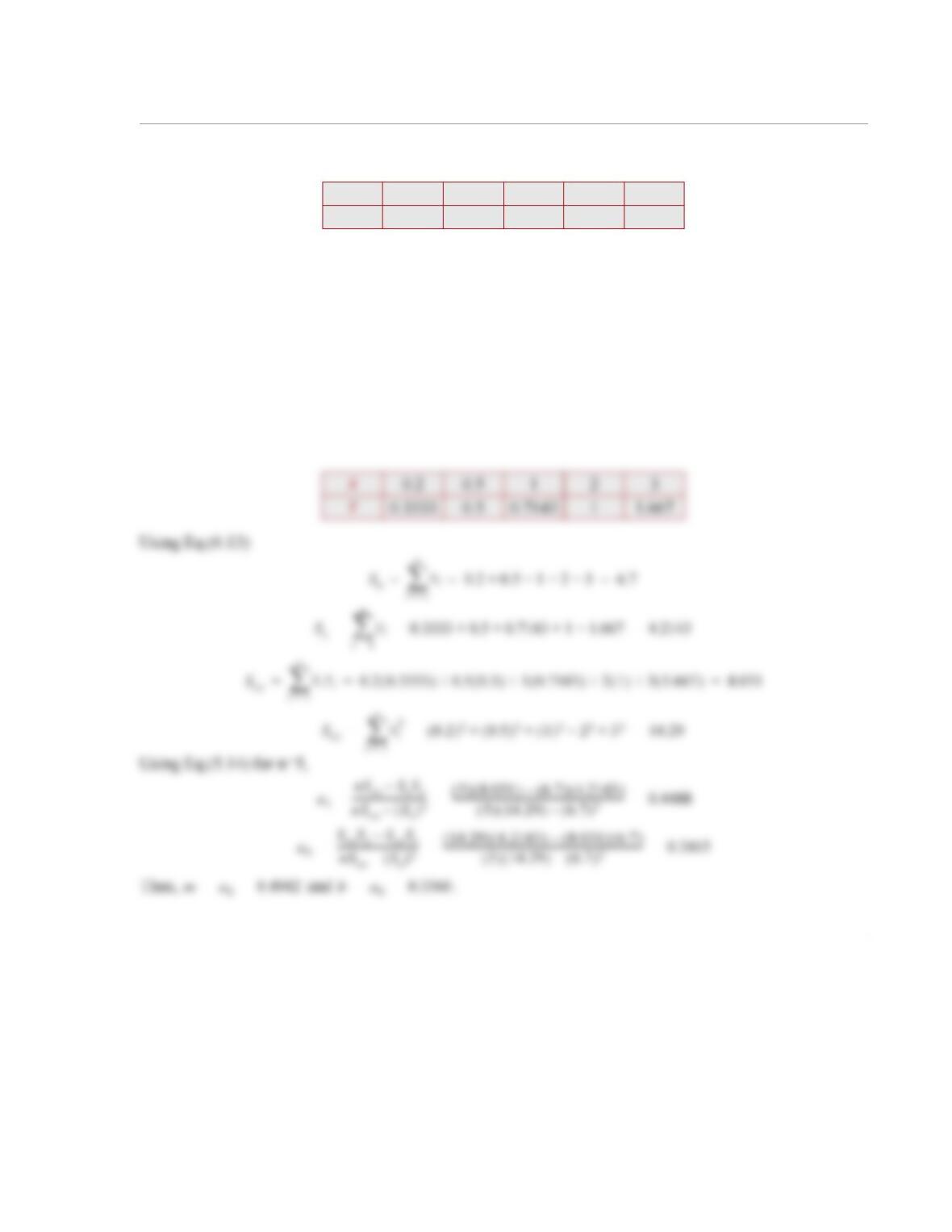
6.4 The following data is given:
Determine the coefficients m and b in the function that best fit the data. Write the equation in
a linear form (Section 6.3), and use linea r least-squares regression to determine the value of the coeffi-
cients.
Solution
The transforming equations from the nonlinear function to the linear form are given in Table
5-2 as , , and . The transformation yields
x0.2 0.5 1 2 3
y3 2 1.4 10.6
y1
mx b+
—————–
=
y1
mx b+
—————–
=
Y1
y
—–
=
Xx=
ma
1
=
ba
0
=
ma
ba
1
6.5 The following data is given:
Determine the coefficients a and b in the function that best fit the data. (Write the function in
a linear form (Section 6.3), and use linea r least-squares regression to determine the value of the coeffi-
cients.) Once the coefficients are determined make a plot that shows the function and the data points.
Solution
The equation is transformed to a linear form:
Linear least square regression is used to find the best fit between and in the form:
x–2 –1 0 1 2
y1.5 3.2 4.5 3.4 2
ya
x2b+
————-–
=
1
y
—–1
a
—–x2b
a
—–
+=
1
y
—–
x2
2
a0=(SXX*SY-SXY*SX)/(n*SXX-SX^2)
a=1/a1
b=a0*a
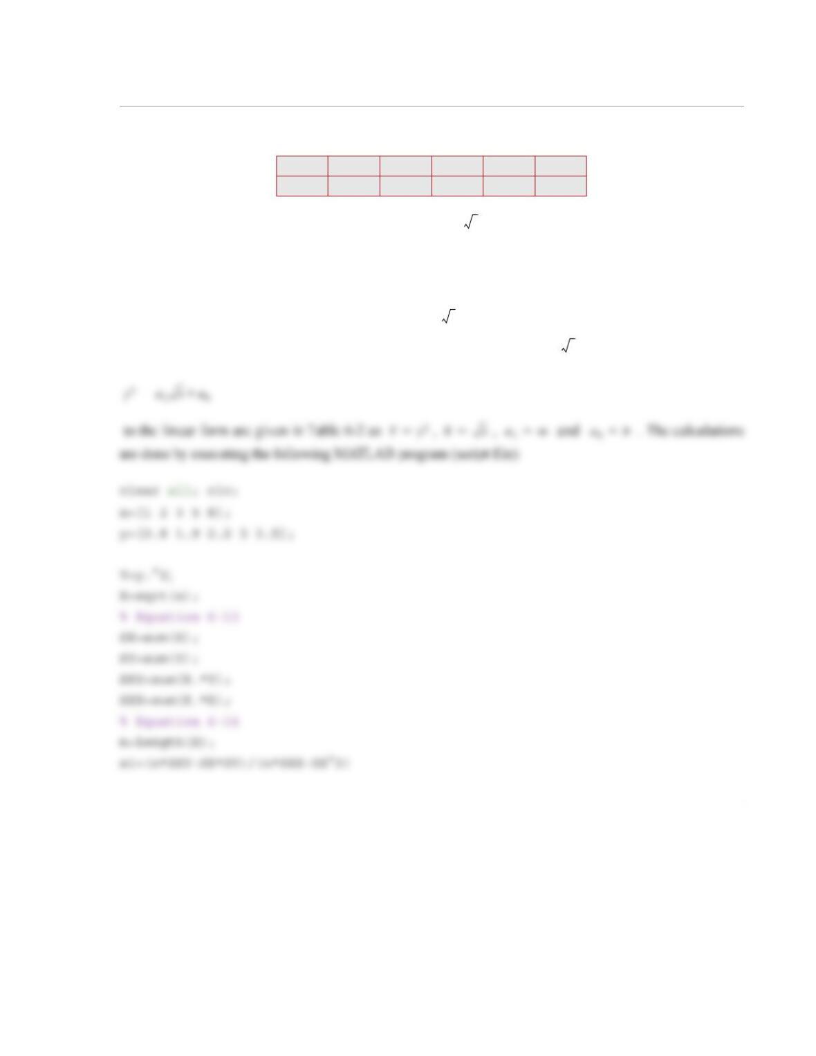
When the program is executed, the following values are displayed in the Command Window:
1
6.6 The following data is given:
Determine the coefficients m and b in the function that best fit the data. Write the equa-
tion in a linear form (Section 6.3), and use linear least-squares regression to determine the value of the
coefficients.
Solution
The equation is transformed to a linear form:
Linear least square regression is used to find the best fit between and in the form:
x12358
y0.8 1.9 2.2 33.5
ymxb+[]
12⁄
=
y2mx b+=
y2
x

2
a0=(SXX*SY-SXY*SX)/(n*SXX-SX^2)
m=a1
b=a0
When the program is executed, the following values are displayed in the Command Window:
a1 =
6.4015
1
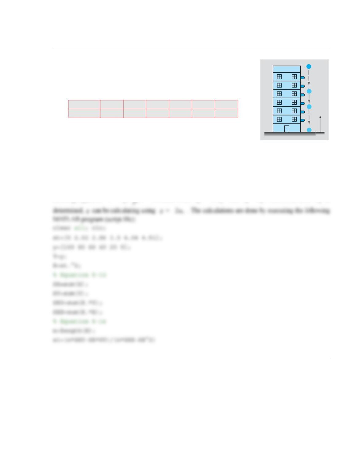
6.7 To measure g (the acceleration due to gravity), the following experi-
ment is carried out. A ball is dropped from the top o f a 100-m-tall building.
As the object is falling down, the time t when it passes sensors mounted on
the building wall is recorded. The data measured in the experiment is given
in the table.
In terms of the coordinates shown in the figure, the position of the ball h as a
function of the time t is given by , where m is the
initial position of the ball. Use linear regression to best fit the equation to the
data and determine the experimental value of g.
Solution
The equation can be transformed into linear form by setting and . The
resulting equation, , is linear w ith and . Therefore, once is
h (m) 100 80 60 40 20 0
t (s) 02.02 2.86 3.50 4.04 4.51 h
hh
0
1
2
—–gt2
–=
h0100=
hh
0
1
2
—–gt2
–=
Yh=
Xt
2
=
Yh
0
1
—–gX–=
a10.5g–=
a0h0
=
a1
2
a0=(SXX*SY-SXY*SX)/(n*SXX-SX^2)
g=-2*a1
h0=a0
When the program is executed, the following values are displayed in the Command Window:
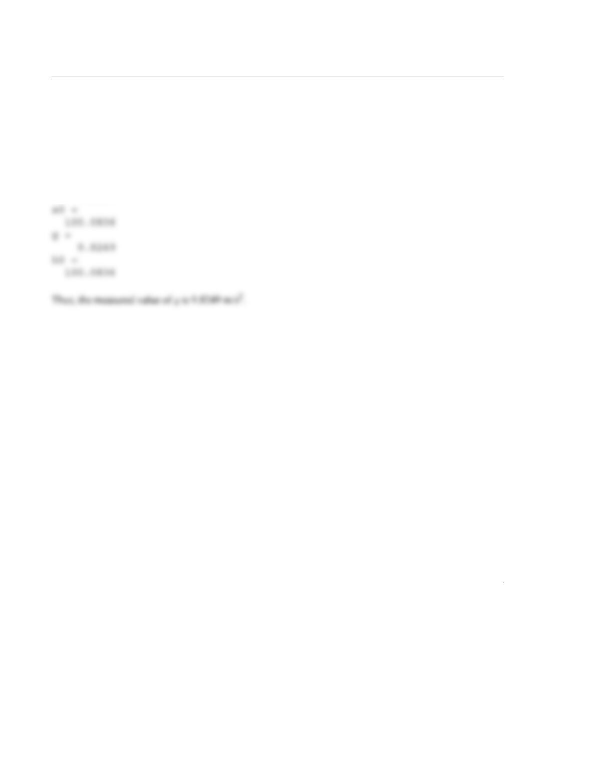
a1 =
-4.9124
1
6.8 Water solubility in jet fuel , , as a function of temperature, T, can be modeled by an exponential
function of the form . The following are values of water solubility measured at different tem-
peratures. Using linear regression, determine the constants m and b that best fit the data. Use the equation
to estimate the water solubility at a temperature of C. Make a plot that shows the function and the data
points.
Solution
The nonlinear function is transferred to a linear function (see Table 6-2) by
substituting , , and . Writing and in terms of and gives
and . The calculations are done by executing the following MATLAB program (script
file):
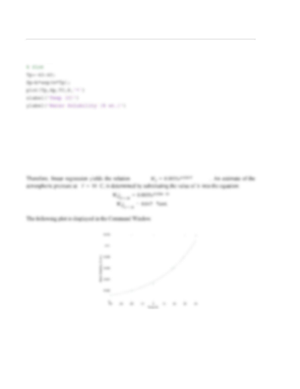
T (oC) –40 –20 020 40
(% wt.) 0.0012 0.002 0.0032 0.006 0.0118
WS
WSbemT
=
10°
WS
WSbemT
=
Ya
1Xa
0
+=
YW
S
ln=
XT=
a1m=
a0bln=
m
b
a1
a0
ma
1
=
be
a0
=
2
% Estimated solubility at 10C
S10=b*exp(m*10)
When the program is executed, the following values are displayed in the Command Window:
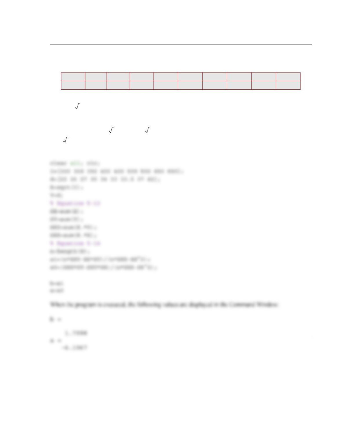
m =
0.0284
b =
0.0035
S10 =
0.0047
1
6.9 In an electrophoretic fiber-making process, the diameter of the fiber, d, is related to the current flow,
I. The following are measured during production:
The relationship between the current and the diameter can be modeled with an equation of the form
. Use the data to determine the constants a and b that best fit the data.
Solution
The equation is linear in and . The coefficients and are found by setting and
and using the method of linear regression. The calculations are done by executing the following
MATLAB program (script file):
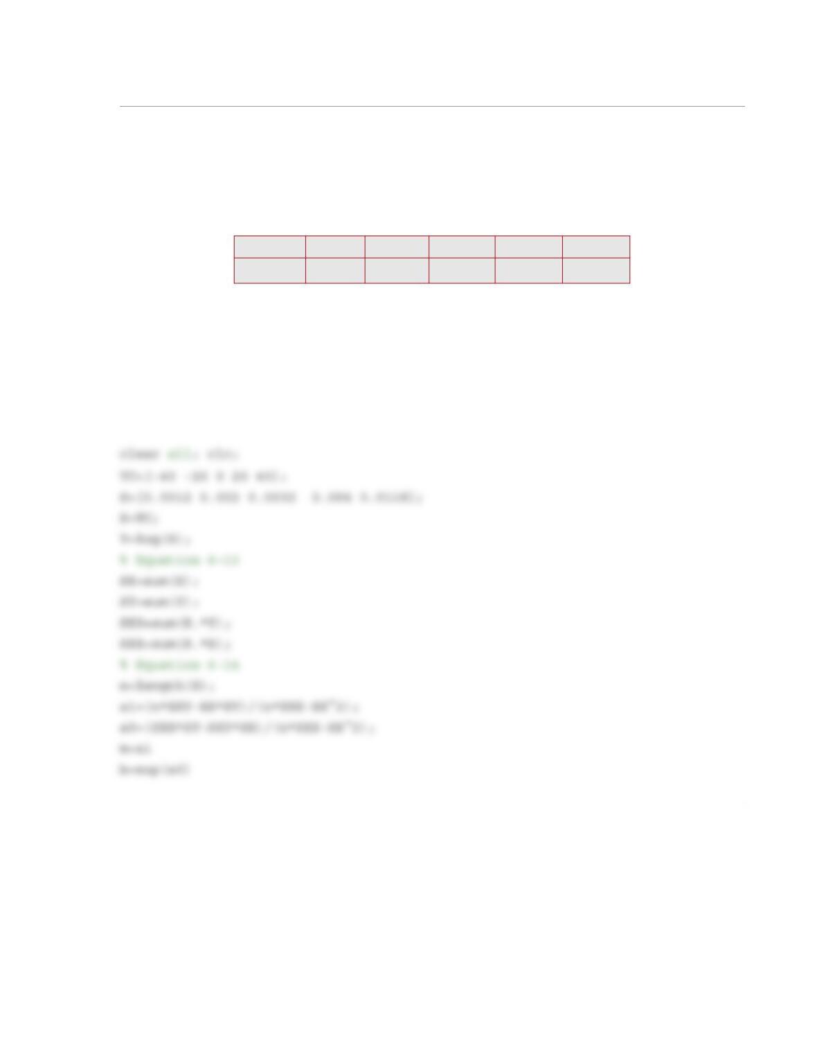
I (nA) 300 300 350 400 400 500 500 650 650
d (µm) 22 26 27 30 34 33 33.5 37 42
dabI+=
dabI+=
I
d
a
b
Yd=
XI=
1
6.10 Determine the coefficients of the polynomial that best fit the data given in Prob-
lem 6.5.
Solution
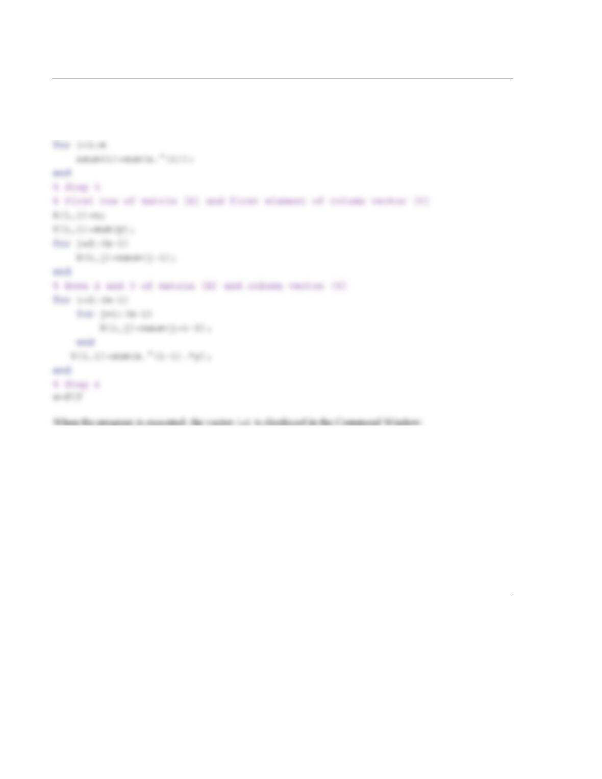
The data points from Problem 6.5 are:
Curve fitting of these data points with the second-order polynomial is done by polynomial regression. The
values of the three coefficients , and are determined by solving a system of three linear equations,
which given by Eqs. (6.26)-(6.28):
x–2 –1 0 1 2
y1.5 3.2 4.5 3.4 2
ya
2x2a1xa
0
++=
a2
a1
a0
2
n=length(x);
m=4;
% Step 2
a =
4.1486
0.1200
-0.6143
The second-order polynomial that best fits the data is .
y0.6143x2
–0.12x4.1486++=
1
6.11 Using the method in Section 6.8, determine the coefficients of the equation that best
fit the following data:
Solution
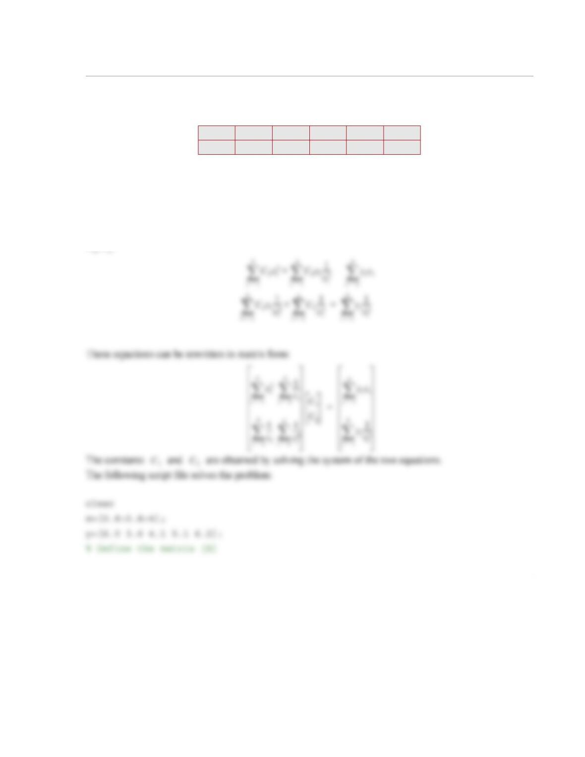
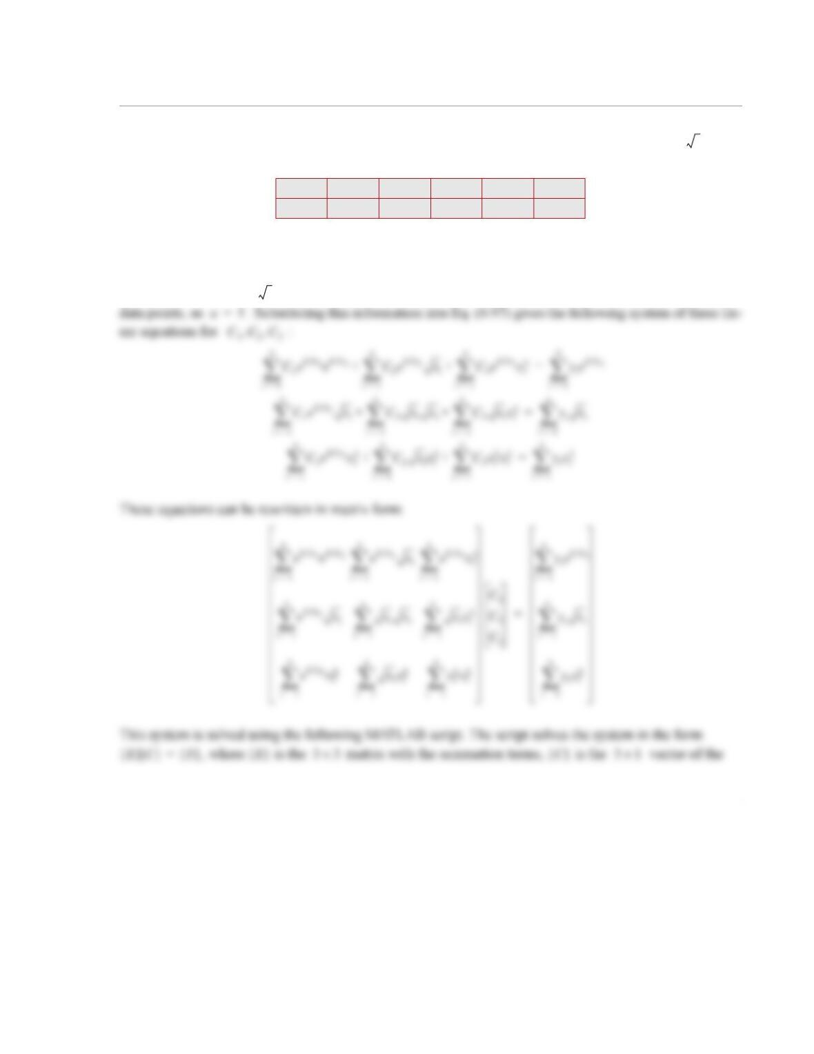
In the notation of Eq. (6.91) the approximating function is , where
and . The equation therefore has two terms, so , and there are five data points, so
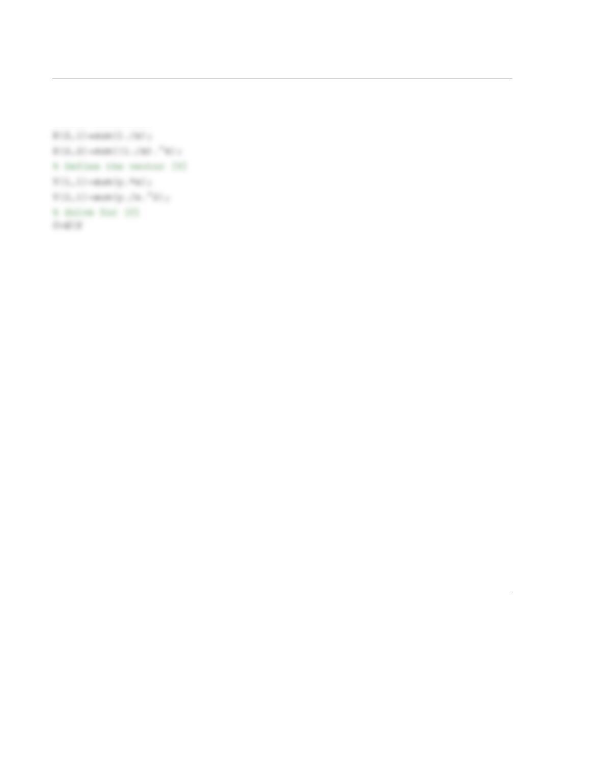
. Substituting this information into Eq. (6.97) gives the following system of two linear equations for
:
x0.8 1.6 2.4 3.2 4.0
y63.6 4.1 5.1 6.2
yaxbx
2
⁄+=
Fx() C1f1x() C2f2x()+=
f1x() x=
f2x() 1
x2
—-–
=
m2=
n5=
C1C2
,
2
X(1,1)=sum(x.^2);
X(1,2)=sum(1./x);
When the script is executed the following result is displayed in the Command Window:
C =
1.4987
3.0714
Thus, the equation that best fit the data is:
y1.4987x3.0714 x2
⁄+=
1
6.12 Using the method in Section 6.8, determine the coefficients of the equation
that best fit the following data:
Solution
In the notation of Eq. (6.91) the approximating function is , where
, and . The equation has three terms, so , and there are five
x0.4 1.0 1.6 2.2 2.8
y5.1 7.1 88.1 7.8
yAe
x2⁄Bx Cx
2
++=
Fx() C1f1x() C2f2x() C3f3x()++=
f1x() e0.5 x
=
f2x() x=
f3x() x2
=
m3=
2
unknowns and is the vector on the right-hand side.
clear all; clc;
x=0.4:0.6:2.8;
y=[5.1 7.1 8 8.1 7.8];
F1=@ (x) exp(x/2);
F2=@ (x) sqrt(x);
F3=@ (x) x.^2;
When the program is executed, the vector is displayed in the Command Window:
c =
1.0991
6.1794
-0.8943
Y[]
31×
C[]
1
6.13 The power generated by a windmill varies with the wind speed. In an experiment, the following five
measurements were obtained:
Determine the fourth-order polynomial in the Lagrange form that passes through the points. Use the poly-
nomial to calculate the power at a wind speed of 26 mph.
Solution
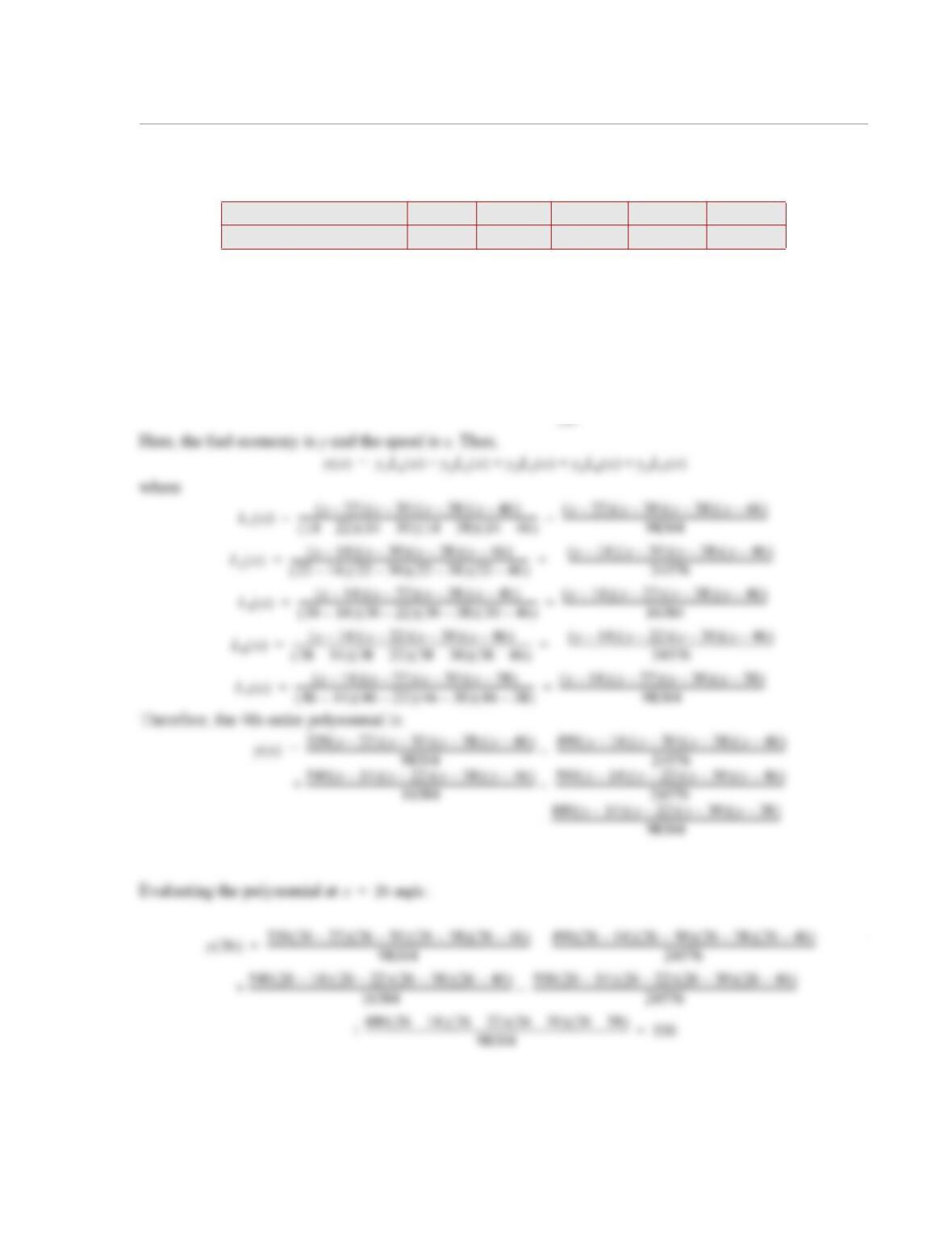
Lagrange polynomials are given by Eq.(5.45):
Wind Speed (mph) 14 22 30 38 46
Electric Power (W) 320 490 540 500 480
fx() yiLix()
i1=
n
yi
xx
j
–()
xixj
–()
—————––
j1=
n
∏
i1=
n
==