4
a=0; b=pi; n=100; Ya=1.5; Yb=0;
WL=-5; WH=-1.5;
When the script file is executed, the following figure is displayed in the Figure Window:
This solution agrees with the solution in Example 11-6.
1
1.5
x
1
11.15 Write a user-defined MATLAB function that uses the finite difference method to solve a second-
order ODE of the form:
for with and
where p, q, and are constants. Discretize the ODE using second-order accurate central differences.
Name the function [x,y]=BVP2ndConst(a,b,n,Ya,Yb,p,q,rOFx). The input arguments a and
b define the domain of the solution, Ya and Yb are the boundary conditions, n is the number of subinter-
vals, and rOFx is a name for the function that calculates . It is a dummy name for the anonymous or
user-defined function that is imported into BVP2ndConst. Within the program, use MATLAB’s left divi-
sion operation to solve the system of linear equations.
Use BVP2ndConst with 50 subintervals to solve the ODE in Problem 11.1 with the boundary con-
ditions , . Plot the solution.
Solution
Using central difference formulas for the derivatives gives:
d2y
dx2
——-–pdy
dx
—––qy++ rx()=
axb≤≤
ya() Ya
=
yb() Yb
=
Ya
Yb
rx()
y0() 1=
y2() 0=
yi1– 2yi
–yi1+
+
—————————————– pyi1+ yi1–
–
2h
—————–——— qyi
++rx
i
()=
2
% d2y/dx2 + p(dy/dx) + qy = r(x)
%using the finite difference method.
%The boundary conditions are assumed to be of the constant Dirichlet form:
% y(a) = Ya and y(b) = Yb
h=(b-a)/n;
A=zeros(n-1,n-1); x(1)=a;
for i=2:n+1
x(i)=x(i-1)+h;
end
% The equation for the first interior point.
A(1,1)=h*h*q-2; A(1,2)=1+h*p/2;
rhs(1)=h*h*rOFx(x(2))-Ya*(1-(h*p/2));
% The equations for interior points: second through one before the last.
3
The ODE that is solved is from Problem 11.1:
In the notation that is used in Problem 11.15:
, , and .
In order to solve the problem, the following user-defined function that calculate , is created:
The following program (script file) solves the problem:
% Solution of Problem 11.15_3ed
clear; clc
d2y
dx2
——––yxsin+=
d2y
dx2
——––yx
2
+=
p0=
q1–=
rx() xsin=
rx()
When the script file is executed, the following figure is displayed in the Figure Window:
0.8
1
1.2
1
1.16 Write a user-defined MATLAB function that uses the finite difference method to solve a boundary
value problem of the form:
for with and
where and are constants. Discretize the ODE using second-order accurate central differences. For
the function name and arguments use [x,y]=BVP2ndVar(a,b,Ya,Yb,n,pOFx,qOFx,rOFx).
The input variables a and b define the domain of the solution, Ya and Yb are the boundary conditions, n is
the number of subintervals, and pOFx, qOFx, and rOFx are the names for the user-defined functions that
calculate , , and , respectively. They are dummy names for the anonymous or user-defined
functions that are imported into BVP2ndVar. Within the program, use MATLAB’s left division operation
to solve the system of linear equations.
Use BVP2ndVar with 50 subintervals to solve the boundary value problem in Problem 11.3. Plot
the solution.
Solution
Using central difference formulas for the derivatives gives:
d2y
dx2
——-–px()
dy
dx
—––qx()y++ rx()=
axb≤≤
ya() Ya
=
yb() Yb
=
Ya
Yb
px()
qx()
rx()
yi1– 2yi
–yi1+
+
h2
—————-——————-—-– px
i
()
yi1+ yi1–
–
2h
—————-———- qx
i
()yi
++rx
i
()=
2
%The function solves a general second order linear ODE of the form:
% d2y/dx2 + p(x)(dy/dx) + q(x)y = r(x)
%using the finite difference method.
%The boundary conditions are assumed to be of the constant Dirichlet form:
% y(a) = Ya and y(b) = Yb
h=(b-a)/n;
A=zeros(n-1,n-1); x(1)=a;
for i=2:n+1
x(i)=x(i-1)+h;
end
% The constants of the equation for the first interior point.
A(1,1)=h*h*qOFx(x(2))-2; A(1,2)=1+h*pOFx(x(2))/2;
rhs(1)=h*h*rOFx(x(2))-Ya*(1-(h*pOFx(x(2))/2));
3
end
% The constants of the equation for the last interior point
A(n-1,n-2)=1-h*pOFx(x(n))/2; A(n-1,n-1)=h*h*qOFx(x(n))-2;
The ODE that is solved is from Problem 9.3:
In the notation that is used in Problem 11.16:
, , and .
In order to solve the problem, the following three user-defined functions that calculate , and
are created:
The following program (script file) solves the problem:
% Solution of Problem 11.16
clear; clc
d2y
dx2
——––xdy
dx
—––y++ 2xy=
px() x=
qx() 12x–=
rx() 0=
px()
qx()
rx()
4
When the script file is executed, the following figure is displayed in the Figure Window:
1.01
1.015
1.02
1.025
1
11.17 Write a user-defined MATLAB function that uses the finite difference method to solve a boundary
value problem of the form (see Eq. (11.24)):
for with and
where and are constants. Discretize the ODE using second-order accurate central differences. For
function name and arguments use [x,y]=BVP2ndDriv(a,b,Ya,Db,n,pOFx,qOFx,rOFx). The
input variables a and b define the domain of the solution, Ya and Db are the boundary conditions, n is the
number of subintervals, and pOFx, qOFx, and rOFx are the names for the user-defined functions that cal-
culate , , and , respectively. Within the program, use MATLAB’s left division operation to
solve the system of linear equations.
Use BVP2ndDriv with 50 subintervals to solve the following boundary value problem:
, ,
Plot the solution.
Solution
Using central difference formulas for the derivatives gives:
d2y
dx2
——-–px()
dy
dx
—––qx()y++ rx()=
axb≤≤
ya() Ya
=
dy
dx
—––
xb=
Db
=
Ya
Db
px()
qx()
rx()
d2y
dx2
——-–1
x
—–dy
dx
—––
+10–=
y1() 1=
dy
dx
—––
x3=
1.2–=
yi1– 2yi
–yi1+
+
—————-——————-—-– px
i
()
yi1+ yi1–
–
—————-———- qx
i
()yi
++rx
i
()=
2
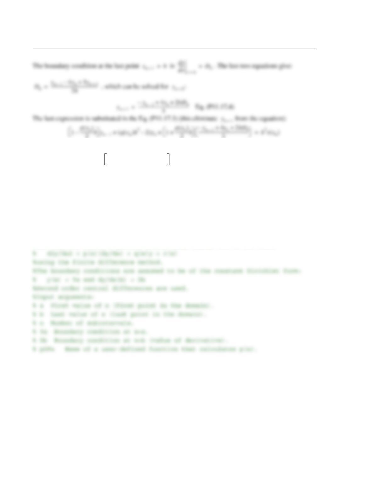
This equation can be written as:
Eq. (P11.17.5)
The solution for is obtained by solving a system of equations made of Eqs. (P11.17.1),
(P11.17.2), and (P11.17.5). Then, the solution at the last point is calculated by Eq. (P11.17.4).
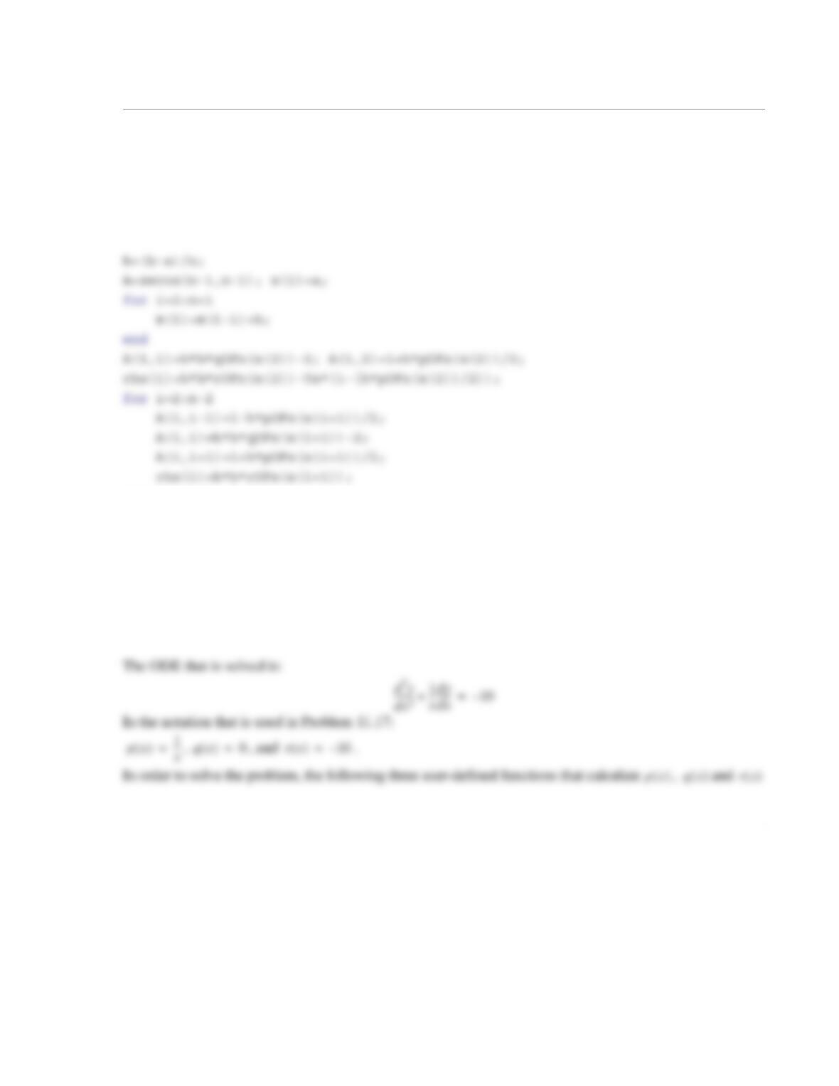
The user-defined function BVP2ndDeriv is listed in the following. Notice that in the program, the system
of linear equations that is solved has equations, and that the ith equation in the system corresponds to
the point in the domain.
function [x,y]=BVP2ndDeriv(a,b,Ya,Db,n,pOFx,qOFx,rOFx)
%The function solves a general second order linear ODE of the form:
2
2
3
2
3
—–1px
n
()h–[]yn1–
2
3
—–
–px
n
()h22
3
—–px
n
()h++ yn
+h2rx
n
() 1px
n
()
2
————–h+
2hDb
3
————–
–=
y2…yn
,,
n1–
yn1+
n1–
i1+
3
% qOFx Name of a user-defined function that calculates q(x).
% rOFx Name of a user-defined function that calculates r(x).
%Output arguments:
% x A vector with the x coordinate of the solution points.
% y A vector with the y coordinate of the solution points.
end
A(n-1,n-2)=2*(1-pOFx(x(n))*h)/3;
A(n-1,n-1)=-2/3+qOFx(x(n))*h*h+2*pOFx(x(n))*h/3;
rhs(n-1)=h*h*rOFx(x(n))-(1+h*pOFx(x(n))/2)*2*h*Db/3;
y=A\rhs’;
y=[Ya; y]
yb=(-y(n-1)+4*y(n)+2*h*Db)/3;
y=[y; yb];
4
are written:
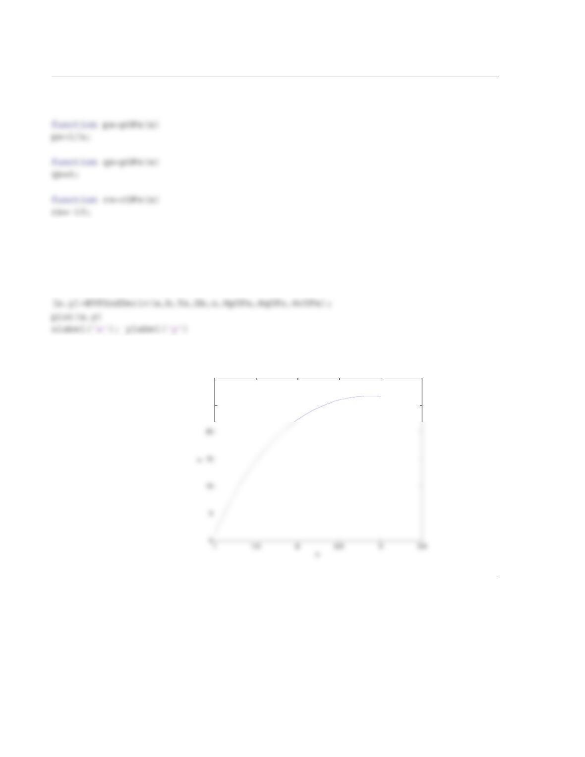
The following program (script file) solves the problem:
% Solution of Problem 11.17
clear all
a=1; b=3; n=50; Ya=1; Db=-1.2;
When the script file is executed, the following figure (solution) is displayed in the Figure Window:
25
30
1
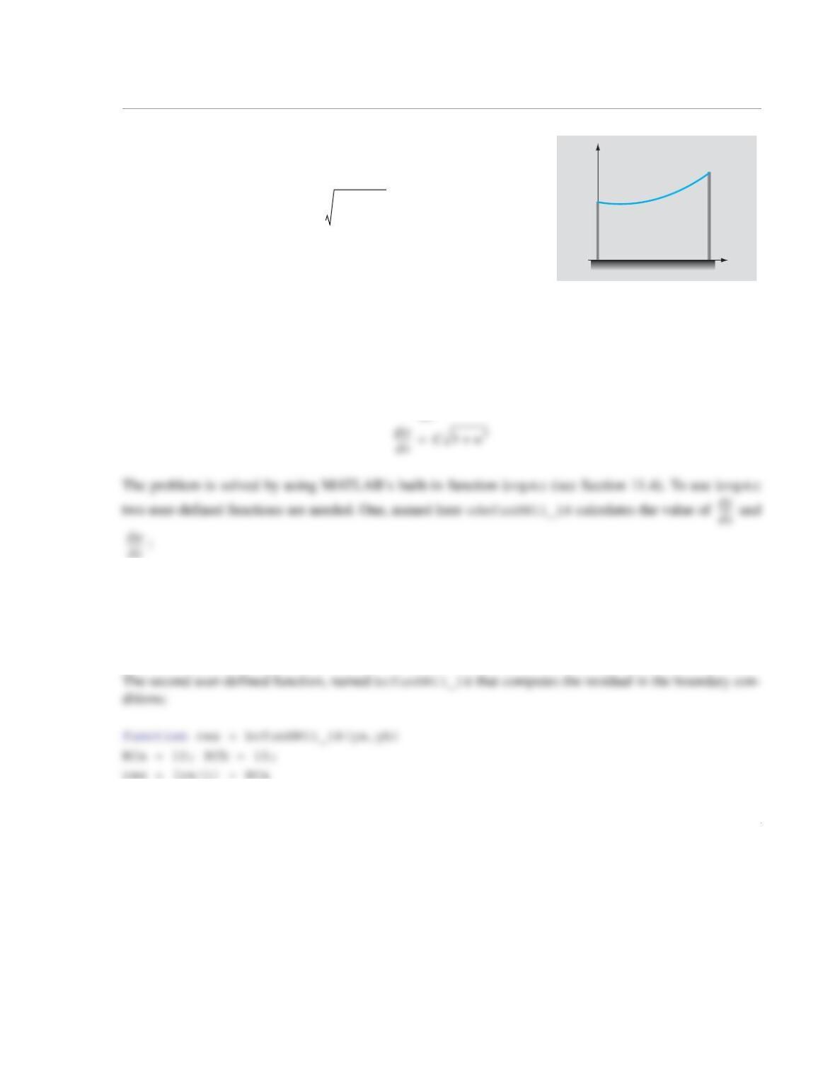
11.18 A flexible cable of uniform density is suspended between two
points, as shown in the figure. The shape of the cable, , is gov-
erned by the differential equation:
where C is a constant equal to the ratio of the weight per unit length
of the cable to the magnitude of the horizontal component of tension
in the cable at its lowest point. The cable hangs between two points
specified by m and m, and m–1.
Use MATLAB’s built-in functions to determine and plot the shape of the cable between and
m.
Solution
The ODE is transforming into a system of two first-order ODEs:
function dydx = odefunHW11_18(x,yw)
C=0.041;
dydx = [yw(2)
C*sqrt(1+yw(2)^2)];
x
y
(0, 10)
(20, 15)
yx()
d2y
dx2
——-–C1dy
dx
—––
2
+=
y0() 10=
y20() 15=
C0.041=
x0=
x20=
dy
dx
—––w=
2
yb(1) – BCb];
The program in the following script file solves the problem:
% Solution of HW 11_18 (script file)
clear, clc
solinit =bvpinit(linspace(0,20,20),[12,12]);
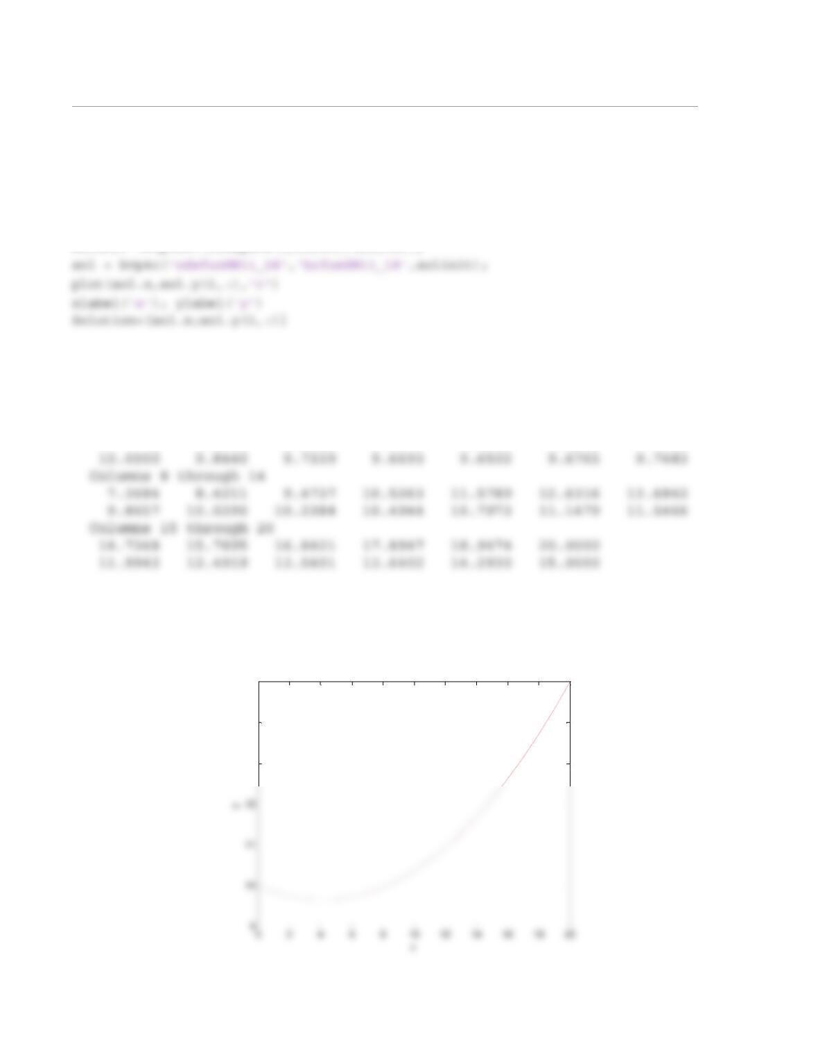
When the script file is executed, the following numerical solution is displayed in the Command Window,
and the following plot of the solution is displayed in the Figure Window:
Solution =
Columns 1 through 7
0 1.0526 2.1053 3.1579 4.2105 5.2632 6.3158
13
14
15
1
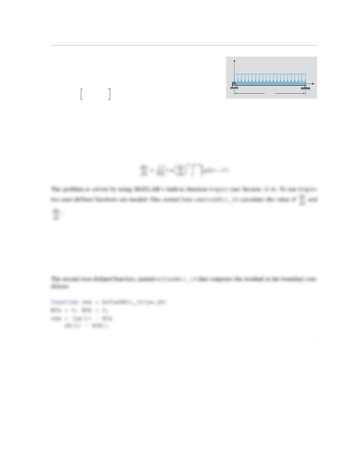
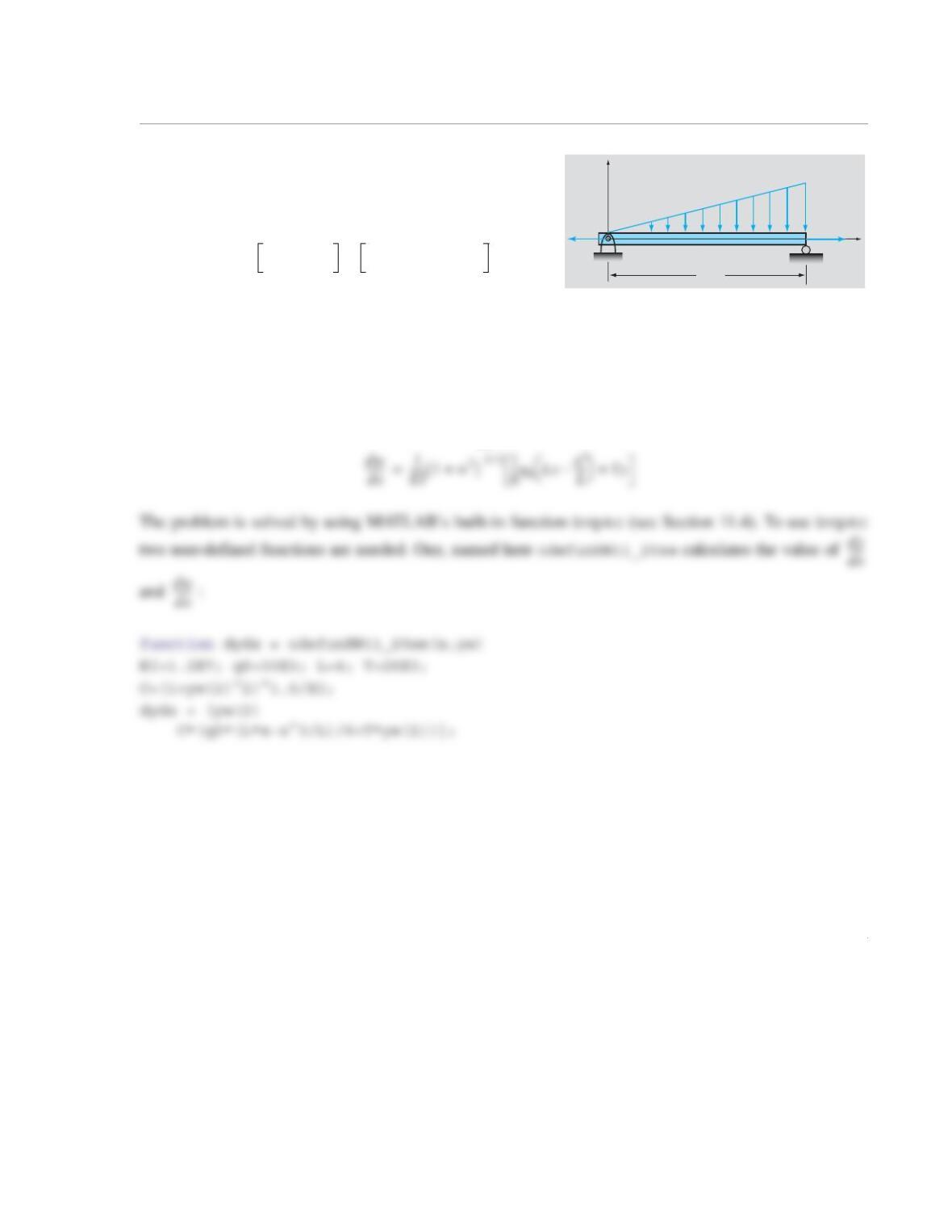
11.19 A simply supported beam of length m is loaded by a
uniform distributed load, as shown in the figure. For large deflec-
tions, the deflection of the beam, y, is determined from the solution
of the following ODE:
and
where N–m2 is the flexural rigidity, and
N/m.
Use MATLAB’s built-in functions to determine and plot the deflection of the beam as a function of x.
Solution
The ODE is transforming into a system of two first-order ODEs:
function dydx = odefunHW11_19(x,yw)
EI=1.4E5; q0=10E3; L=4;
C=q0/(2*EI);
dydx = [yw(2)
C*(L*x-x^2)*(1+yw(2)^2)^1.5];
x
y
q
L
L4=
EI d2y
dx2
——-–1dy
dx
—––
2
+
32⁄1
2
—–qLx x
2
–()=
y0() 0=
yL() 0=
EI 1.4 107
×=
q10 103
×=
dy
dx
—––w=
2
The program in the following script file solves the problem:
% Solution of HW11_19 (Script file)
clear
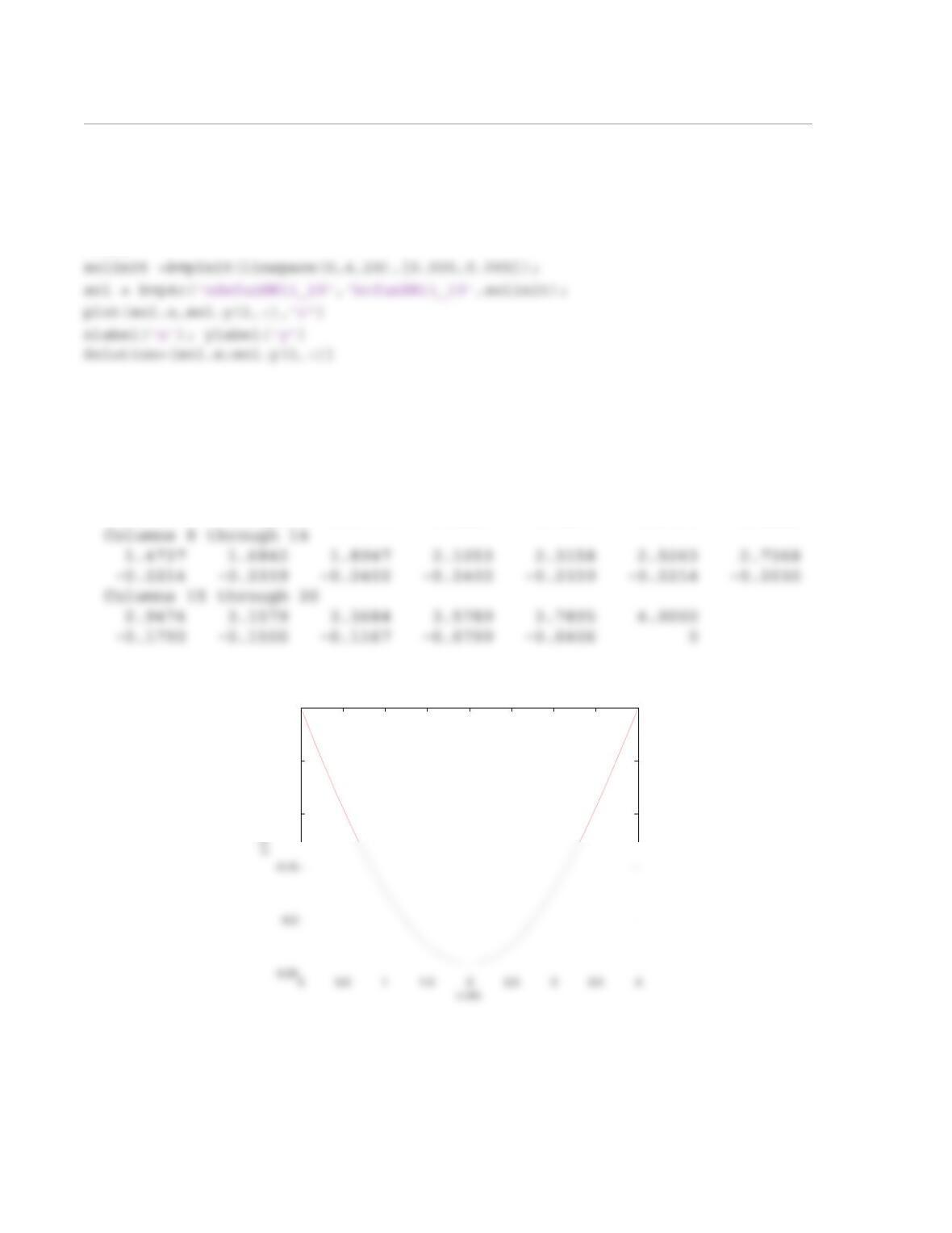
When the script file is executed, the following numerical solution is displayed in the Command Window,
and the following plot of the solution is displayed in the Figure Window:
Solution =
Columns 1 through 7
0 0.2105 0.4211 0.6316 0.8421 1.0526 1.2632
0 -0.0406 -0.0799 -0.1167 -0.1500 -0.1790 -0.2030
-0.1
-0.05
0
1
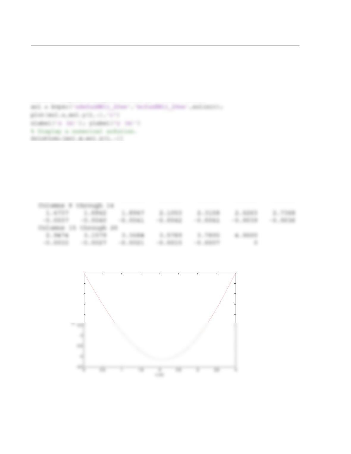
11.20 A simply supported beam of length m is
loaded by a distributed load and a tensile axial force T, as
shown in the figure. The deflection of the beam, y, is deter–
mined from the solution of the following ODE:
with the boundary conditions and .
N–m2 is the flexural rigidity, N/m, and N.
Use MATLAB’s built-in functions to determine and plot the deflection of the beam as a function of x.
Solution
The ODE is transforming into a system of two first-order ODEs:
The second user-defined function, named bcfunHW11_20se that computes the residual in the boundary
conditions:
function res = bcfunHW11_20se(ya,yb)
BCa = 0; BCb = 0;
res = [ya(1) – BCa
yb(1) – BCb];
x
y
T
L
q0
T
L4=
d2y
dx2
——-–1
EI
—––1dy
dx
—––
2
+
32⁄1
6
—–q0Lx x3
L
—-–
–
Ty+=
y0() 0=
yL() 0=
EI 1.2 107
×=
q030 103
×=
T20 103
×=
dy
dx
—––w=
2
The program in the following script file solves the problem:
% Solution of HW11_20se (Script file)
clear, clc
solinit =bvpinit(linspace(0,4,20),[-0.005,-0.005]);
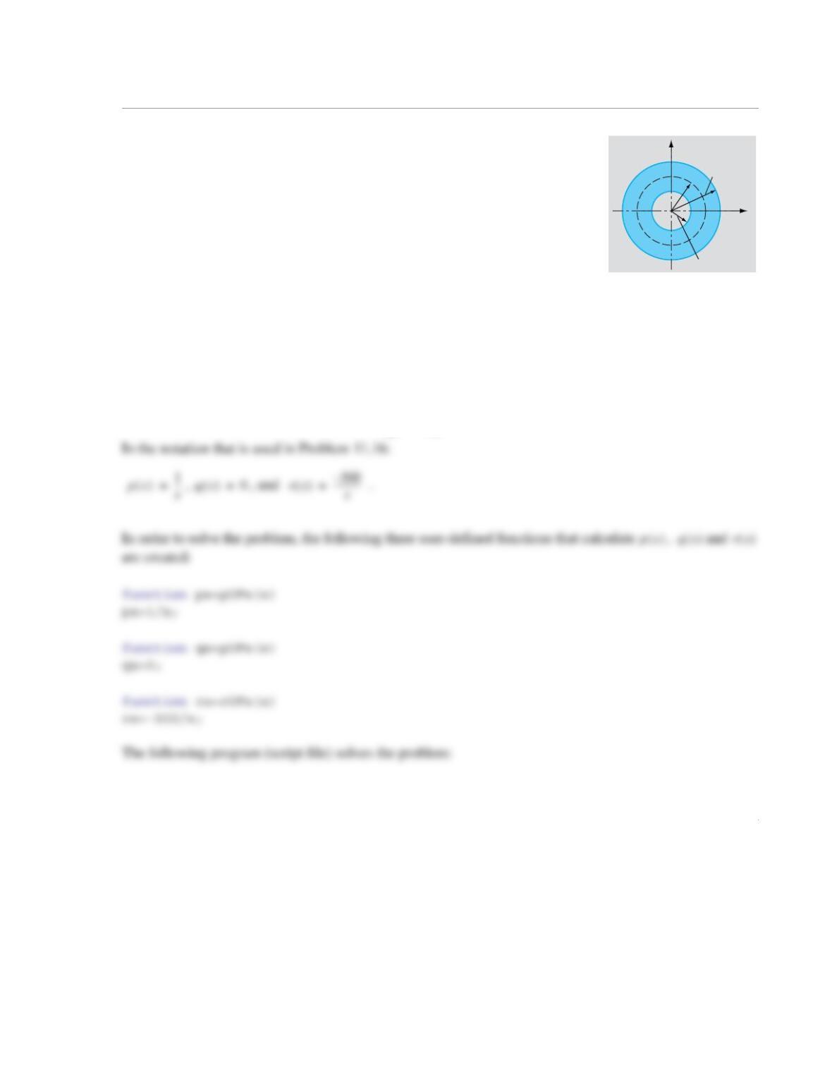
When the script file is executed, the following numerical solution is displayed in the Command Window,
and the following plot of the solution is displayed in the Figure Window:
Solution =
Columns 1 through 7
0 0.2105 0.4211 0.6316 0.8421 1.0526 1.2632
0 -0.0007 -0.0013 -0.0019 -0.0024 -0.0029 -0.0034
-2
-1.5
-1
-0.5
0x 10-3
1
11.21 A cylindrical pipe with inner radius 1 cm and wall thickness 2.5 cm car–
ries a fluid at a temperature of 600oC. The outer wall of the pipe is at 25oC.
The governing equation for the temperature distribution in the pipe wall is:
subject to the boundary conditions oC and oC. Solve
for the temperature and plot the temperature distribution as a function of
r.
(a) Use the user-defined function BVP2ndVar (written in Problem 11.16) with 5 subintervals.
(b) Use the user-defined function BVP2ndVar (written in Problem 11.16) with 10 subintervals.
(c) Use MATLAB built-in functions to solve the ODE.
Solution
(a) The ODE that is solved is:
x
y
35 mm
r
10 mm
rd2T
dr2
———– dT
dr
—––
+ 500–=
T1() 600=
T3.5() 25=
Tr()
d2T
dr2
———– 1
r
—–dT
dr
—––
+ 500–=
2
% Solution of Problem 11.21
clear, clc,
a=1; b=3.5; n=5; Ya=600; Yb=25;
[x,y]=BVP2ndVar(a,b,Ya,Yb,n,@pOFx,@qOFx,@rOFx);
plot(x,y)
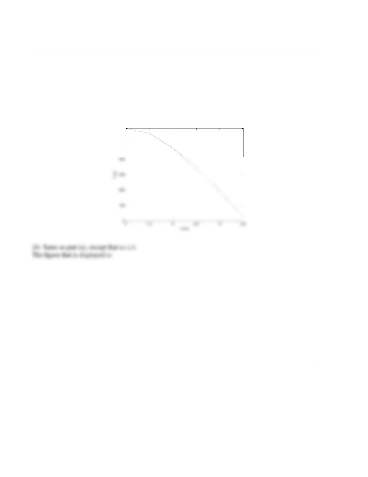
xlabel(‘r’); ylabel(‘T (C)’)
When the script file is executed, the following figure is displayed in the Figure Window:
500
600