1
10.1 Consider the following first-order ODE:
from to with
(a) Solve with Euler’s explicit method using .
(b) Solve with the modified Euler method using .
(c) Solve with the classical fourth-order Runge–Kutta method using .
The analytical solution of the ODE is . In each part, calculate the error between the true
solution and the numerical solution at the points where the numerical solution is determined.
Solution
(a) The following script file solves the ODE with Euler’s explicit method using .
dy
dx
—––x2y⁄=
x0=
x2.1=
y0() 2=
h0.7=
h0.7=
h0.7=
y2x3
3
——-–4+=
h0.7=
2
error =
0 0.0564 0.2429 0.3863
(b) The following script file solves the ODE with modified Euler method using .
clear, clc
% Solving the ODE with the modified Euler’s method.
clear,clc
dF=@ (x,y) x^2/y;
Fsol=@ (x) sqrt(2*x.^3/3+4);
When the program is executed, the following results are displayed in the Command Window:
x =
0 0.7000 1.4000 2.1000
h0.7=
3
(c) The following script file solves the ODE with classical fourth-order Runge–Kutta method using
.
% Solving the ODE with the classical fourth-order Runge-Kutta method.
h=0.7; N=3;
x(1) = 0; y(1) = 2;
for i = 1:N
x(i+1) = x(i) + h;
end
x
y
ys=Fsol(x);
error=ys-y
When the program is executed, the following results are displayed in the Command Window:
h0.7=
1
10.2 Consider the following first-order ODE:
from to with
(a) Solve with Euler’s explicit method using .
(b) Solve with the modified Euler method using .
(c) Solve with the classical fourth-order Runge–Kutta method using .
The analytical solution of the ODE is . In each part, calculate the error between the true
solution and the numerical solution at the points where the numerical solution is determined.
Solution
(a) The following script file solves the ODE with Euler’s explicit method using .
% Solving the ODE with Euler’s explicit method.
clear,clc
end
x
y
ys=Fsol(x);
error=ys-y
When the program is executed, the following results are displayed in the Command Window:
dy
dx
—––xxy
2
—-–
–=
x1=
x3.4=
y1() 1=
h0.8=
h0.8=
h0.8=
y2e
1x2
–
4
————-–
–=
h0.8=
2
error =
0 0.0288 -0.0689 -0.0781
(b) The following script file solves the ODE with modified Euler method using .
% Solving the ODE with the modified Euler’s method.
clear,clc
dF=@ (x,y) x-x*y/2;
end
x
y
ys=Fsol(x);
error=ys-y
When the program is executed, the following results are displayed in the Command Window:
x =
1.0000 1.8000 2.6000 3.4000
h0.8=
3
.
% Solving the ODE with the classical fourth-order Runge-Kutta method.
clear,clc
h=0.8; N=3;
x(1) = 1; y(1) = 1;
for i = 1:N
x(i+1) = x(i) + h;
end
x
y
ys=Fsol(x);
error=ys-y
When the program is executed, the following results are displayed in the Command Window:
h0.8=
1
10.3 Consider the following first-order ODE:
from to with
(a) Solve with Euler’s explicit method using .
(b) Solve with the midpoint method using .
(c) Solve with the classical fourth-order Runge–Kutta method using .
The analytical solution of the ODE is . In each part, calculate the error between
the true solution and the numerical solution at the points where the numerical solution is determined.
Solution
(a) The following script file solves the ODE with Euler’s explicit method using .
% Solving the ODE with Euler’s explicit method.
end
t
y
ys=Fsol(t);
error=ys-y
When the program is executed, the following results are displayed in the Command Window:
dy
dt
—––yt
3
+=
t0=
t1.5=
y0() 1=
h0.5=
h0.5=
h0.5=
y7ett3
–3t2
–6t–6–=
h0.5=
2
0 0.1660 0.7155 2.2781
(b) The following script file solves the ODE with midpoint method using .
% Solving the ODE with midpoint method.
t(i+1) = t(i) + h;
tm = t(i) + h/2;
ym=y(i) + dF(t(i),y(i))*h/2;
y(i+1) = y(i) + (dF(tm,ym))*h;
end
t
y
ys=Fsol(t);
error=ys-y
When the program is executed, the following results are displayed in the Command Window:
h0.5=
3
% Solving the ODE with the classical fourth-order Runge-Kutta method.
t(i+1) = t(i) + h;
K1= dF(t(i),y(i));
K2= dF(t(i)+0.5*h,y(i)+K1*h/2);
K3= dF(t(i)+0.5*h,y(i)+K2*h/2);
K4= dF(t(i+1),y(i)+K3*h);
y(i+1) = y(i) + (K1+2*K2+2*K3+K4)*h/6;
When the program is executed, the following results are displayed in the Command Window:
1
10.4 Consider the following first-order ODE:
from to with
(a) Solve with Euler’s explicit method using .
(b) Solve with the modified Euler method using .
(c) Solve with the classical third-order Runge–Kutta method using .
The analytical solution of the ODE is . In each part, calculate the error between the true
solution and the numerical solution at the points where the numerical solution is determined.
Solution
(a) The following script file solves the ODE with Euler’s explicit method using .
% 3ed Chapter 10 Problem 4 Part (a)
% Solving the ODE with Euler’s explicit method.
When the program is executed, the following results are displayed in the Command Window:
t =
2 3 4 5
dy
dt
—––y
t
— 0.5t2
–=
t2=
t5=
y2() 4=
h1=
h1=
h1=
yt3
4
—–
–3t+=
h1=
2
(b) The following script file solves the ODE with modified Euler method using .
% Solving the ODE with the modified Euler’s method.
clear,clc
dF=@ (x,y) x-x*y/2;
Fsol=@ (x) 2-exp((1-x.^2)/4);
When the program is executed, the following results are displayed in the Command Window:
t =
2 3 4 5
h1=
3
(c) The following script file solves the ODE with classical fourth-order Runge–Kutta method using
.
% Solving the ODE with the classical fourth-order Runge-Kutta method.
clear,clc
end
t
y
ys=Fsol(t);
error=ys-y
When the program is executed, the following results are displayed in the Command Window:
t =
2 3 4 5
h1=
1
10.5 Consider the following system of two ODEs:
from to with , and
(a) Solve with Euler’s explicit method using .
(b) Solve with the modified Euler method using .
The analytical solution of the system is , . In each part, calculate
the error between the true solution and the numerical solution at the points where the numerical solution is
determined.
Solution
(a) The following script file solves the system of the ODEs with Euler’s explicit method using .
clear, clc
a=0; b=1.2;
dx
dt
—––2x2y+=
dy
dt
—––2xy–=
t0=
t1.2=
x0() 1=
y0() 2=
h0.4=
h0.4=
xe2t–8e5t3–()
5
——————————-–
=
y2e2t–2e5t3+()
5
————————————–
=
h0.4=
2
Yerror=soly(t)-y
When the program is executed, the following results are displayed in the Command Window:
t =
0 0.4000 0.8000 1.2000
(b) The following script file solves the system of the ODEs with the modified Euler method using
.
clear, clc
a=0; b=1.2;
dxdt = @ (x,y) 2*x+2*y;
h0.4=
3
y(i+1) = y(i) + (dydt(x(i),y(i))+dydt(xEU,yEU))*h/2;
end
When the program is executed, the following results are displayed in the Command Window:
t =
0 0.4000 0.8000 1.2000
x =
1.0000 4.3600 13.4800 39.7510
1
10.6 Consider the following system of two ODEs:
from to with , and
(a) Solve with Euler’s explicit method using .
(b) Solve with the classical fourth-order Runge–Kutta method using .
The analytical solution of the system is , . In each part, calcu-
late the error between the true solution and the numerical solution at the points where the numerical solu-
tion is determined.
Solution
(a) The following script file solves the system of the ODEs with Euler’s explicit method using .
clear, clc
a=0; b=1.2;
h = 0.4;
N=3;
for i = 1:N
t(i+1) = t(i) + h;
x(i+1) = x(i) + dxdt(x(i),y(i),t(i))*h;
dx
dt
—––xyt–=
dy
dt
—––ty+=
t0=
t1.2=
x0() 1=
y0() 1=
h0.4=
h0.4=
x4ett2et
–t2
–3t–3–=
y2ett–1–=
h0.4=
2
When the program is executed, the following results are displayed in the Command Window:
t =
0 0.4000 0.8000 1.2000
(b) The following script file solves the system of the ODEs with the classical fourth-order Runge–Kutta
method using .
clear, clc
a=0; b=1.2;
dxdt = @ (t,x,y) x-y*t;
dydt = @ (t,x,y) t+y;
h0.4=
3
Kx3= dxdt(t(i)+0.5*h,x(i)+Kx2*h/2,y(i)+Ky2*h/2);
end
t
x
y
Xerror=solx(t)-x
Yerror=soly(t)-y
When the program is executed, the following results are displayed in the Command Window:
t =
0 0.4000 0.8000 1.2000

1
10.7 Write the following second-order ODE as a system of two first-order ODEs:
Solution
d2y
dt2
——-– 5dy
dt
—––
2
6y–etsin
++0=
1
10.8 Write the following second-order ODEs as systems of two first-order ODEs:
(a) , where E, I, P, Q, and L are constants.
(b) , where E, I, and M are constants.
Solution
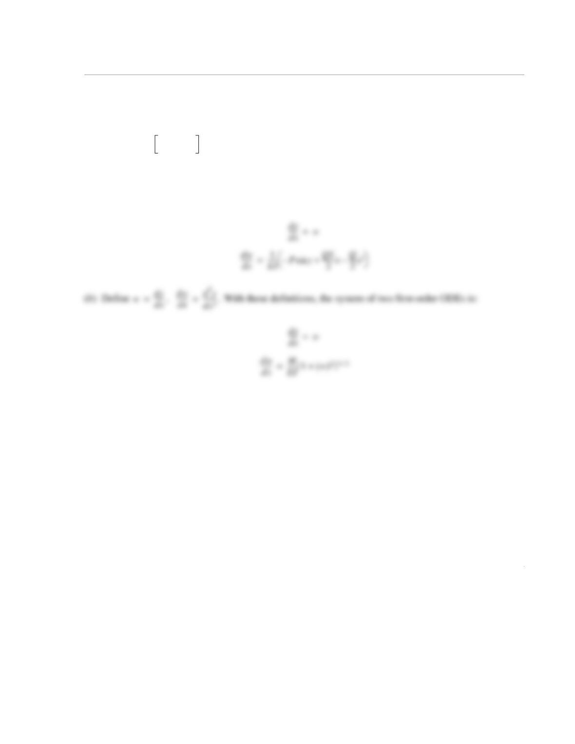
(a) Define , . With these definitions, the system of two first-order ODEs is:
EI d2y
dx2
——––Pysin–QL
2
——-–xQ
2
—–x2
–+=
EI d2y
dx2
——––M1dy
dx
—––
2
+
32⁄
=
wdy
dx
—––
=
dw
dx
——–d2y
dx2
——-–
=
wdy
dx
dw
dx
——–d2y