1
10.9 Write the following second-order ODEs as systems of two first-order ODEs:
(a), where g, T, and w are constants.
(b).
Solution
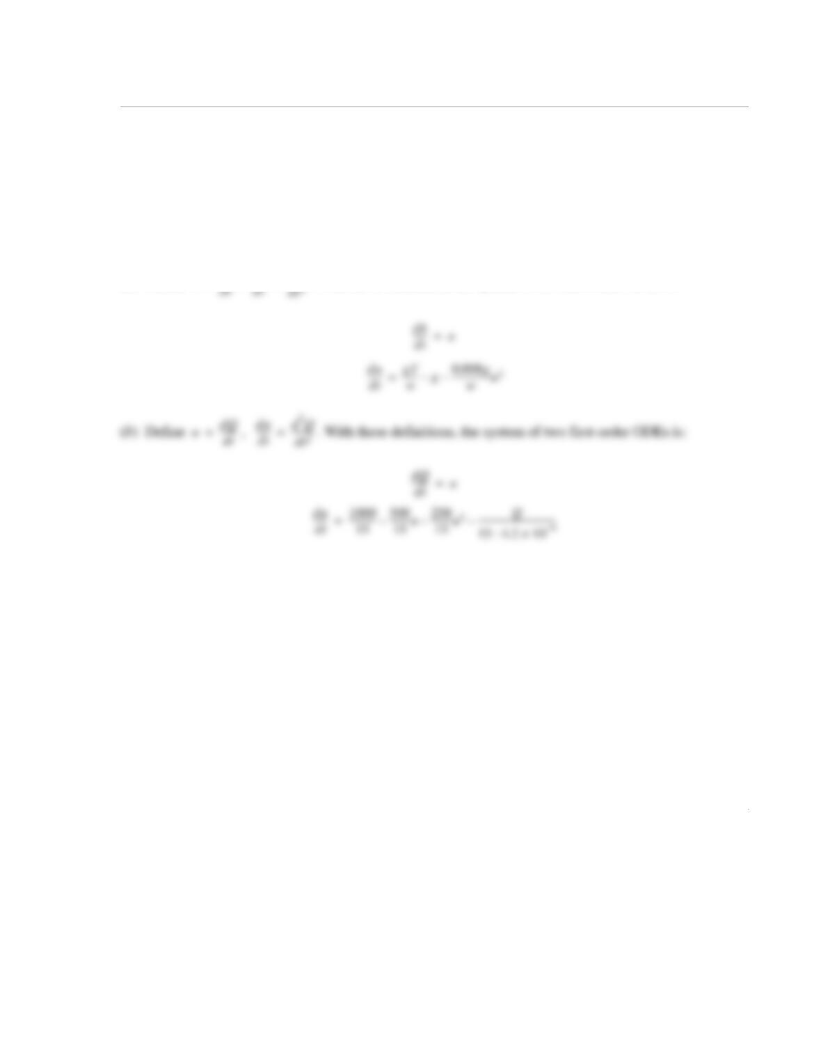
(a) Define , . With these definitions, the system of two first-order ODEs is:
1
g
—–d2h
dt2
——––T
w
—–1– 0.008
w
————– dh
dt
—––
2
–=
d2Q
dt2
———– 500
15
——––dQ
dt
——– 250
15
——––dQ
dt
——–
3Q
15 4.2 10 6–
×⋅
—————–—————–
++ + 1000
15
———––
=
udh
—––
=
du
—––d2h
——-–
=
1
10.10 Write the following system of two second-order ODEs as a system of four first-order ODEs:
Solution
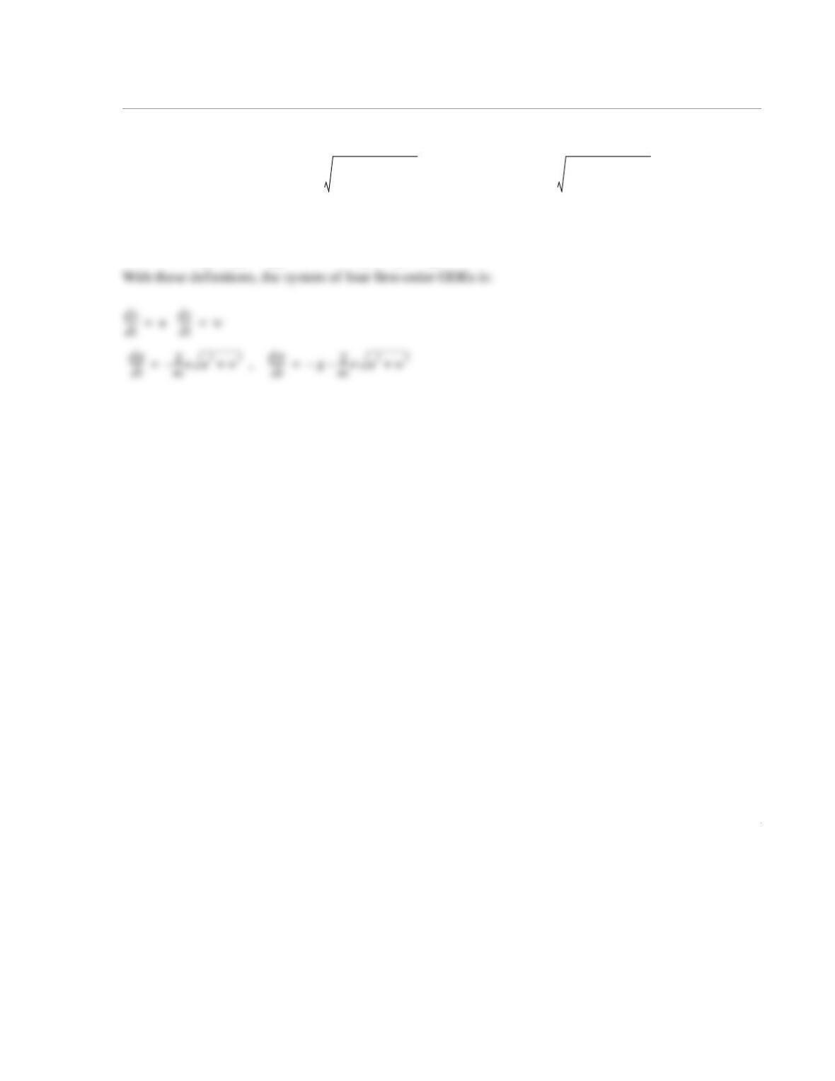
Define , , and ,
d2x
dt2
——––γ
m
—–dx
dt
—––
dx
dt
—––
2dy
dt
—––
2
+–=
d2y
dt2
——––g–γ
m
—–dy
dt
—––
dx
dt
—––
2dy
dt
—––
2
+–=
wdy
dt
—––
=
dw
dt
——–d2y
dt2
——-–
=
udx
dt
—––
=
du
dt
—––d2x
dt2
——-–
=
1
10.11 Consider the following second-order ODE:
from to , with and
(a) Solve with Euler’s explicit method using .
(b) Solve with the modified Euler method using .
The analytical solution of the ODE is . In each part, calculate the error
between the true solution and the numerical solution at the points where the numerical solution is deter-
mined.
Solution
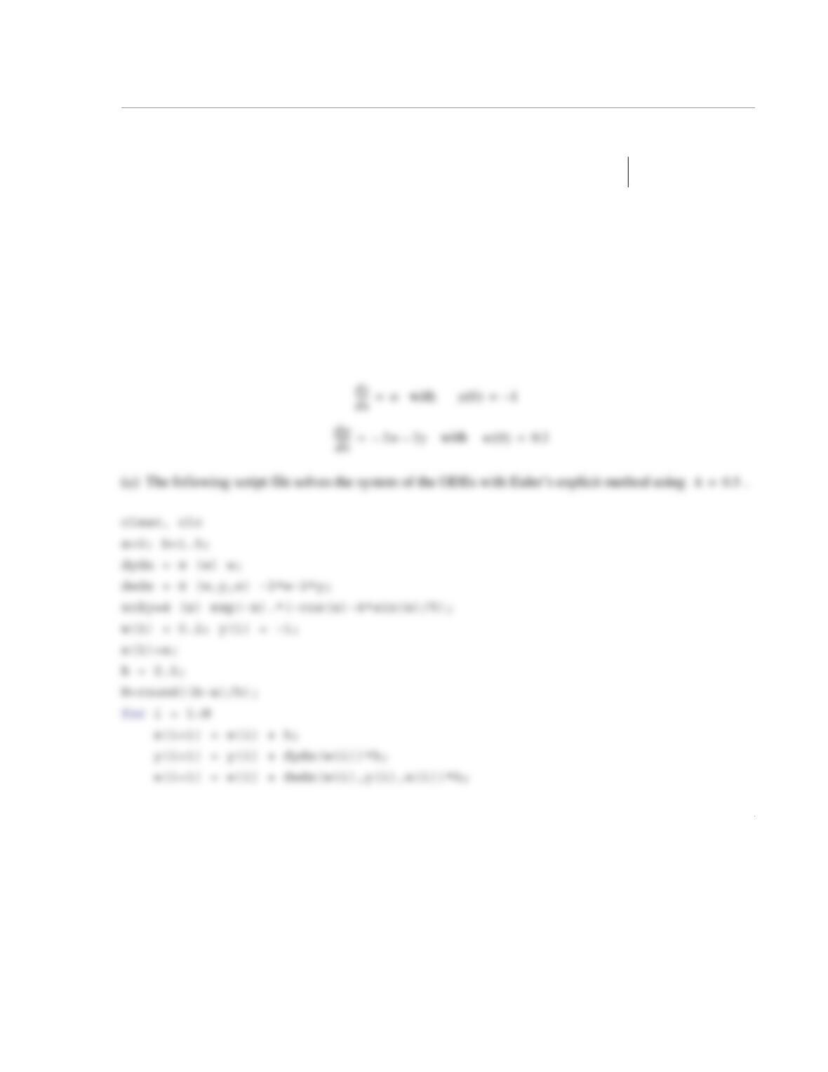
Define , . With these definitions, the system of two first-order ODEs is:
d2y
dx2
——––2dy
dx
—––2y++ 0=
x0=
x1.5=
y0() 1–=
dy
dx
—––
x0=
0.2=
h0.5=
h0.5=
ye
x–x()cos–4x()5⁄sin–()=
wdy
dx
—––
=
dw
dx
——–d2y
dx2
——-–
=
2
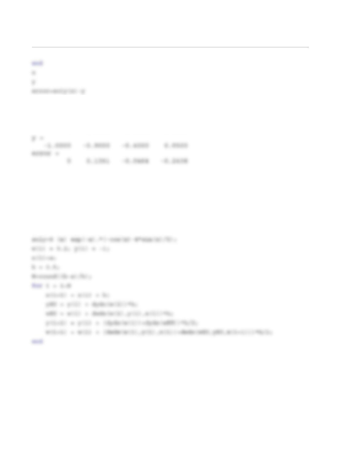
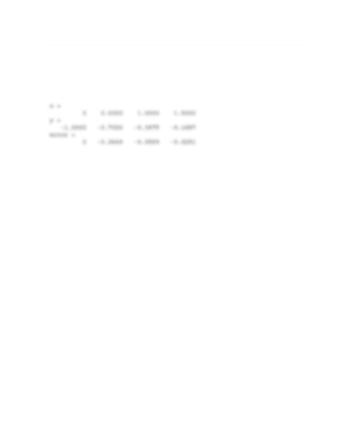
When the program is executed, the following results are displayed in the Command Window:
x =
0 0.5000 1.0000 1.5000
(b) The following script file solves the system of the ODEs with the modified Euler method using
.
clear, clc
a=0; b=1.5;
dydx = @ (w) w;
dwdx = @ (w,y,x) -2*w-2*y;
h1=
3
x
y
error=soly(x)-y
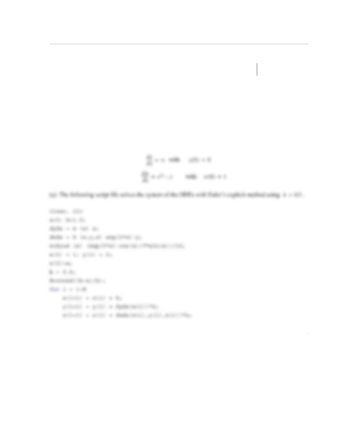
When the program is executed, the following results are displayed in the Command Window:
1
10.12 Consider the following second-order ODE:
from to , with and
(a) Solve with Euler’s explicit method using .
(b) Solve with the classical fourth-order Runge–Kutta method using .
The analytical solution of the ODE is . In each part, calculate the error
between the true solution and the numerical solution at the points where the numerical solution is deter-
mined.
Solution
Define , . With these definitions, the system of two first-order ODEs is:
d2y
dx2
——––e3xy–=
x0=
x1.5=
y0() 0=
dy
dx
—––
x0=
1=
h0.5=
h0.5=
ye
3xx()cos–7x()sin+()10⁄=
wdy
dx
—––
=
dw
dx
——–d2y
dx2
——-–
=
2
end
x
y
error=soly(x)-y
When the program is executed, the following results are displayed in the Command Window:
x =
0 0.5000 1.0000 1.5000
(b) The following script file solves the system of the ODEs with the classical fourth-order Runge–Kutta
method using .
clear, clc
a=0; b=1.5;
dydx = @ (w) w;
h0.5=
3
end
x
y
error=soly(x)-y
When the program is executed, the following results are displayed in the Command Window:
x =
0 0.5000 1.0000 1.5000
y =
1
10.13 Consider the following second-order ODE:
from to , with and
(a) Solve with Euler’s explicit method using .
(b) Solve with the classical fourth-order Runge–Kutta method using .
mined.
Solution
Define , . With these definitions, the system of two first-order ODEs is:
with
with
(a) The following script file solves the system of the ODEs with Euler’s explicit method using .
clear, clc
a=0; b=1;
dydx = @ (w) w;
d2y
dx2
——––exy–
=
x0=
x1.0=
y0() 0=
dy
dx
—––
x0=
1=
h0.5=
h0.5=
wdy
dx
—––
=
dw
dx
——–d2y
dx2
——-–
=
dy
dx
—––w=
y0() 0=
dw
dx
——–exy–
=
w0() 1=
h0.5=
2
When the program is executed, the following results are displayed in the Command Window:
(b) The following script file solves the system of the ODEs with the classical fourth-order Runge–Kutta
method using .
clear, clc
a=0; b=1;
dydx = @ (w) w;
dwdx = @ (w,y,x) exp(-x*y);
w(1) = 1; y(1) = 0;
x(1)=a;
h = 0.5;
N=round((b-a)/h);
for i = 1:N
h0.5=
end
x
y
When the program is executed, the following results are displayed in the Command Window:
1
10.14 Use the user-defined MATLAB function odeEULER (Program 10-1 which is listed in Example 10-
1) to solve Problem 10.1. Write a MATLAB program as a script file that solves the ODE in Problem 10.1
three times, once by using , once by using , and once by using . The program
should also plot the exact solution (given in Problem 10.1) and plot the three numerical solutions (all in the
same figure).
Solution
The listing of the user-defined function odeEULER is:
x(1) = a; y(1) = yINI;
N = round((b-a)/h);
for i = 1:N
x(i+1) = x(i) + h;
y(i+1) = y(i) + ODE(x(i),y(i))*h;
end
The user-defined function odeEULER is used in following program (in a script file) solves the problem.
h0.7=
h0.35=
h0.1=
2
h1=0.7; h2=0.35; h3=0.1;
[x1, y1] = odeEULER(ODEHW10_1,a,b,h1,yINI);
[x2, y2] = odeEULER(ODEHW10_1,a,b,h2,yINI);
[x3, y3] = odeEULER(ODEHW10_1,a,b,h3,yINI);
fplot(‘sqrt(2*x^3/3+4)’,[0 2.1])
hold on
plot(x1,y1,‘o’,x2,y2,‘s’,x3,y3,‘*’)
hold off
When the program is executed the numerical solution is displayed in the Command Window and the fol-
lowing plot is displayed in the Figure Window:
Numerical solution with h=0.7
Answer =
0 0.7000 1.4000 2.1000
2.0000 2.0000 2.1715 2.8033
Numerical solution with h=0.35
Answer =
3
2.0451
Columns 9 through 16
2.4607
Columns 17 through 22
1.6000 1.7000 1.8000 1.9000 2.0000 2.1000
2.5522 2.6525 2.7614 2.8787 3.0041 3.1373
3
3.2
3.4
Exact
h=0.7
h=0.35
h=0.1
1
10.15 Use the user-defined MATLAB function odeEULER (Program 10-1 which is listed in Example 10-
1) to solve Problem 10.2. Write a MATLAB program as a script file that solves the ODE in Problem 10.2
three times, once by using , once by using , and once by using . The program
should also plot the exact solution (given in Problem 10.2) and plot the three numerical solutions (all in the
same figure).
Solution
The listing of the user-defined function odeEULER is:
function [x, y] = odeEULER(ODE,a,b,h,yINI)
% odeEULER solves a first order initial value ODE using Euler’s
x(1) = a; y(1) = yINI;
N = round((b-a)/h);
for i = 1:N
x(i+1) = x(i) + h;
y(i+1) = y(i) + ODE(x(i),y(i))*h;
end
The the user-defined function odeEULER is used in following program (in a script file) solves the problem.
h0.8=
h0.4=
h0.1=
2
h1=0.8; h2=0.4; h3=0.1;
[x1, y1] = odeEULER(ODEHW10_2,a,b,h1,yINI);
[x2, y2] = odeEULER(ODEHW10_2,a,b,h2,yINI);
[x3, y3] = odeEULER(ODEHW10_2,a,b,h3,yINI);
When the program is executed the numerical solution is displayed in the Command Window and the fol-
lowing plot is displayed in the Figure Window:
Numerical solution with h=0.8
Answer =
1.0000 1.8000 2.6000 3.4000
1.0000 1.4000 1.8320 2.0067
3
1.7000 1.8000 1.9000 2.0000 2.1000 2.2000 2.3000
1.3755 1.4286 1.4800 1.5294 1.5765 1.6210 1.6627
2
2.2
2.4
Exact
h=0.8
h=0.4
h=0.1
1
10.16 Write a user-defined MATLAB function that solves a first-order ODE by applying the midpoint
method (use the form of second-order Runge–Kutta method, Eqs. (10.65), (10.66)). For function name and
arguments use [x,y]=odeMIDPOINT(ODE,a,b,h,yINI). The input argument ODE is a name for
the function that calculates . It is a dummy name for the function that is imported into odeMIDPOINT.
The arguments a and b define the domain of the solution, h is the step size, and yINI is the initial value.
The output arguments, x and y, are vectors with the x and y coordinates of the solution.
Use the function odeMIDPOINT to solve the ODE in Problem 10.2. Write a MATLAB program in a
script file that solves the ODE twice, once by using and once by using . The program
should also plot the exact solution (given in Problem 10.2) and plot the two numerical solutions (all in the
same figure).
Solution
The listing of the user-defined function odeMIDPOIN is:
function [x, y] = odeMIDPOINT(ODE,a,b,h,yINI)
% odeMIDPOINT solves a first order initial value ODE using the
dy
dx
—––
h0.8=
h0.1=
2
The the user-defined function odeMIDPOIN is used in following program (in a script file) solves the prob-
lem:
clear, clc
ODEHW10_2 = @ (x,y) x-x*y/2;
a=1; b=3.4; yINI=1;
h1=0.8; h2=0.1;
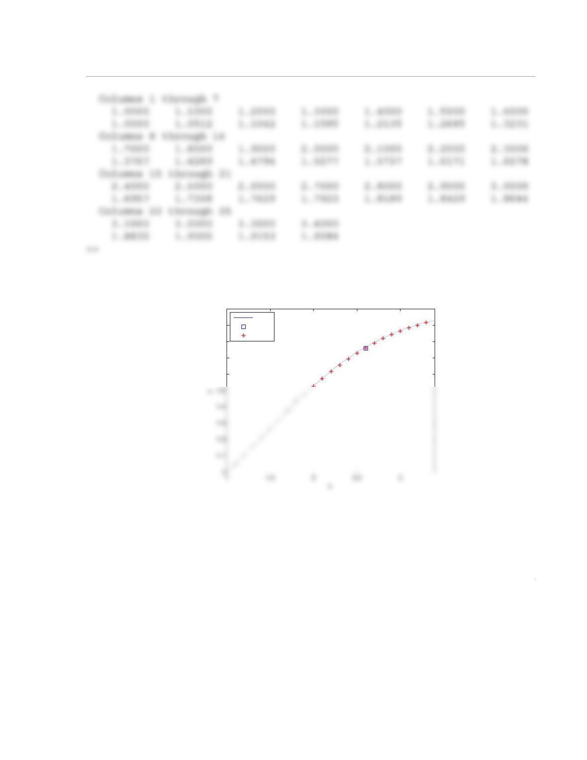
When the program is executed the numerical solution is displayed in the Command Window and the fol-
lowing plot is displayed in the Figure Window:
Numerical solution with h=0.8
Answer =
1.0000 1.8000 2.6000 3.4000
3
1.6
1.7
1.8
1.9
2
Exact
h=0.8
h=0.1
1
10.17 Write a user-defined MATLAB function that solves a first-order ODE by applying the classical
third-order Runge–Kutta method, Eqs. (10.82), (10.83). For function name and arguments use
[x,y]=odeRK3(ODE,a,b,h,yINI). The input argument ODE is a name for the function that calcu-
lates . It is a dummy name for the function that is imported into odeRK3. The arguments a and b define
the domain of the solution, h is the step size, and yINI is the initial value. The output arguments, x and y,
are vectors with the x and y coordinates of the solution.
Use the function odeRK3 to solve Problem 10.2. Write a MATLAB program in a script file that
solves the ODE in Problem 10.2 twice, once by using and once by using . The program
should also plot the exact solution (given in Problem 10.2) and plot the two numerical solutions (all in the
same figure).
Solution
The listing of the user-defined function odeRK3 is:
function [x, y] = odeRK3(ODE,a,b,h,y1)
% odeRK3 solves a first order initial value ODE using Ronge-Kutta third
% order method.
x(1) = a; y(1) = y1;
n = (b-a)/h;
for i = 1:n
dy
dx
—––
h0.8=
h0.1=