Chapter 6 Homework Once And Are Calculated And Are Determined

3

y=[0 3 4.5 5.8 5.9 5.8 6.2 7.4 9.6 15.6 20.7 26.7 31.1 35.6 39.3 41.5];

n=length(x);

[a,Er] = CubicPolyFit(x,y)

When the program is executed, the following plot is displayed in the Figure Window:

35

40

45

Strain ε

Data

Polynomial fit

1

6.24 Write a MATLAB user-defined function for interpolation with natural cubic splines. Name the func-

tion Yint = CubicSplines(x,y,xint), where the input ar guments x and y are vectors with the

coordinates of the data points, and xint is the x coordinate of the interpolated point. The output argument

Yint is the y value of the interpolated point.

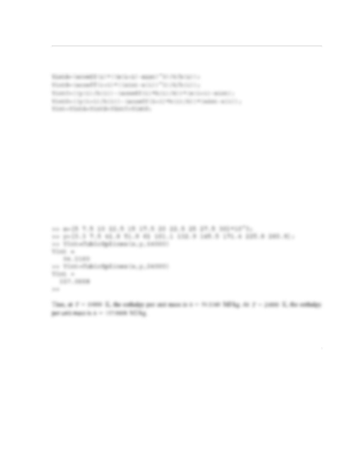
(a) Use the function with the data in Example 6-8 for calculating the interpolated value at .

(b) Use the function with the data in Problem 6.39 for calc ulating the enthalpy per unit mass at

K and at K.

Solution

The listing of the user-defined function CubicSplines is:

function Yint=CubicSplines(x,y,xint)

% CubicSplines fits a set of cubic splines to n data points and then

x12.7=

T14000=

T24000=

2

for i=1:n-3

a(i)=h(i+1);

end

A(1,2)=a(1); A(1,1)=d(1); A(n-2,n-3)=b(n-2); A(n-2,n-2)=d(n-2);

a(1)=a(1)/d(1);

r(1)=r(1)/d(1);

for i=2:n-3

denom=d(i)-b(i)*a(i-1);

if(denom==0), error(‘zero in denominator’), end

a(i)=a(i)/denom;

r(i)=(r(i)-b(i)*r(i-1))/denom;

3

end

i=interval;

(a) The user-defined function CubicSplines is used in the Command Window to calculate the interpo-

lated value at for the data in Example 6-8:

>> x=[8 11 15 18 22];

>> y=[5 9 10 8 7];

>> Yint=CubicSplines(x,y,12.7)

Yint =

10.1189

>>

(b) The user-defined function is used in the Command Window to calculate the enthalpy per unit mass at

K and at K using the data from Problem 6.39:

x12.7=

T14000=

T24000=

1

6.25 Write a MATLAB user-defined function for spline interpolation that uses third-order Lagrange poly-

nomials. Name the function Yint = CubicLagSplines(x,y,xint), where the input arguments x

and y are vectors with the coordinates of the data points, and xint is the x coordinate of the interpolated

point. The output argument Yint is the y value of the interpolated point. The function uses the following

scheme for the interpolation. If xint is in the first interval of the data points, the function uses a second-

order polynomial that passes through the first three data points. If xint is in the last interval of the data

points, the function uses a second-order polynomial that passes through the last three data points. If xint

is in any other int erval, lets say interval i between point and point , the function uses a third-order

polynomial for the interpolation. The third-order polynomial is written such that it passes through the data

points: , , , and .

(a) Use the CubicLagSplines function with the data in Problem 6.13 to calculate the power at wind

speeds of 26 mph and 42 mph.

(b) Use the CubicLagSplines function with the data in Example 6- 3 to calculate the stress at strains

of 0.2 and 3.

Solution

The listing of the user-defined function CubicLagSplines is:

function Yint=CubicLagSplines(x,y,Xint)

xi

xi1+

xi1–

xi

xi1+

xi2+

2

ya=y(i-2:i+1);

Yint=LagrangeINT(xa,ya,Xint);

end

n = length(x);

for i = 1:n

L(i) = 1;

for j = 1:n

if j ~= i

L(i)= L(i)*(Xint-x(j))/(x(i)-x(j));

end

3

Pfor42=CubicLagSplines(S,P,42)

When executes the following results are displayed in the Command Window:

Pfor26 =

(b) A script file that solves Part (b):

Stress3=CubicLagSplines(Strain,Stress,3)

When executes the following results are displayed in the Command Window:

Stress02 =

1.6875

Stress3 =

8.200

1

6.26 A linear combination of three functions that is used for curve fitting has the form (see Section 6.8):

Write a MATLAB user-defined function that determines the coefficients , , and that best fits a

given set of data points. Name the function C = NonLinCombFit(F1,F2,F3,x,y), where the input argu-

ments F1, F2, and F3 are handles of the three functions (user-defined or anonymous) , , and

, and x and y are vectors with the coordinates of the data points. The output argument C is a three-

element row vector with the values of the coefficients , , and .

Use NonLinCombFit to solve Problem 6.40 (a). Write a program in a script file that uses NonLinComb-

Fit and plots the data points and the curve of that best fits the data.

Solution

The listing of the user-defined function NonLinCombFits is:

function c = NonLinCombFit(F1,F2,F3,x,y)

% NonLinComdFit determines the three coefficients C1, C2, C3 of the function

Fx() C1f1x() C2f2x() C3f3x()++=

C1

C2

C3

f1x)()

f2x)()

f3x)()

C1

C2

C3

Fx()

2

a(3,3)=sum(F3(x).*F3(x));

A script file that solves Part (a) of Problem 6.40:

clear; clc

T=[595 623 761 849 989 1076 1146 1202 1382 1445 1562];

When executes the following results are displayed in the Command Window:

c =

1.0e+003 *

-0.052442723579328

0.002121597543987

3.815341691904303

1

6.27 The resistance R of a tungsten wire as a function of temperature can be modeled with the e quation

, where is the resistance corresponding to temperature , and is the tempera-

ture coefficient of resistance. Determine and such that the equation will best fit the following data.

Use C.

(a) Use the user-defined function LinReg developed in Problem 6.19.

(b) Use MATLAB’s built-in function polyfit.

Solution

Rewriting the equation:

Linear regression form:

Thus: and or:

T (C) 20 100 180 260 340 420 500

R () 500 676 870 1060 1205 1410 1565

RR

01αTT

0

–()+[]=

R0

T0

α

R0

α

T020°=

°

Ω

RαR0TR

01αT0

–()+=

Ra

1Ta

0

+=

a1αR0

=

a0R01αT0

–()=

a0R0a1T0

–=

2

T=[20 100 180 260 340 420 500];

R=[500 676 870 1060 1205 1410 1565];

p=polyfit(T,R,1);

R0=p(2)+p(1)*T0

Alpha=p(1)/R0

When the script is executed the following results are displayed in the Command Window:

R0 =

1

6.28 Bacteria growth rate can be modele d with the equation , where is the

growth rate constant, and and are the numbers of bacteria at times t and , respectively. Determine

and such that the equation will best fit the following data. Use .

(a) Use the user-defined function LinReg developed in Problem 6.19.

(b) Use MATLAB’s built-in function polyfit.

Solution

Rewriting the equation:

Linear regression form:

t (h) 0 2 4 6 8

N (cells/ml) 35 1990 70,800 2,810,000 141,250,000

Nt

ln N0

ln–µtt

0

–()=

µ

Nt

N0

t0

µ

N0

t00=

Nt

ln µtN

0

ln µt0

–+=

ya

1ta

0

+=

2

A script file that solves Part (b):

clear, clc

t0=0;

When the script is executed the following results are displayed in the Command Window:

mu =

1.883709642829710

1

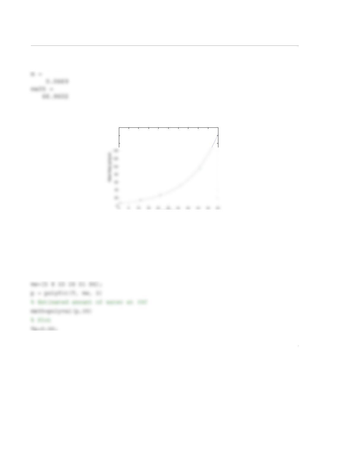
6.29 The amount of water in air measure d at various temperatures at 100% humidity is displayed in the

following table:

(a) Determines the coef ficients of an exponential function of the f orm that best fi ts the

data. Use the function to estimate the amount of water at 35 C. If available, use the user-defined function

ExpoFit developed in Problem 6.20. In one figure, plot the exponential function and the data points.

(b) Use MATLAB’s built-in function polyfit to determine the coefficients of a second-order polyno-

mial that best fits the data. Use the polynomial to estimate the amount of water at 35 C. In one figure, plot

the polynomial and the data points.

Solution

Part (a)

The following script file uses the user-defined function ExpoFit developed in Problem 6.20 to solve the

problem:

(C) 010 20 30 40 50

(g/Kg of air) 5 8 15 28 51 94

T

°

mwater

mwater bemT

=

°

2

b =

6.4494

Figure Window:

Part (b)

The following script file uses the user-defined function ExpoFit developed in Problem 6.20 to solve the

problem:

T=[0 1:10:50];

160

180

200

Temp (C)

3

mp=polyval(p,Tp);

plot(Tp,mp,T,mw,‘*’)

xlabel(‘Temp (C)’)

ylabel(‘Water Mass (g/Kg air)’)

When the script is executed the following is displayed:

Command Window:

p =

0.0547 -0.1696 7.2549

mw35 =

1

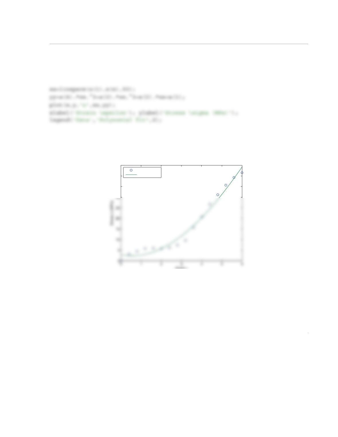
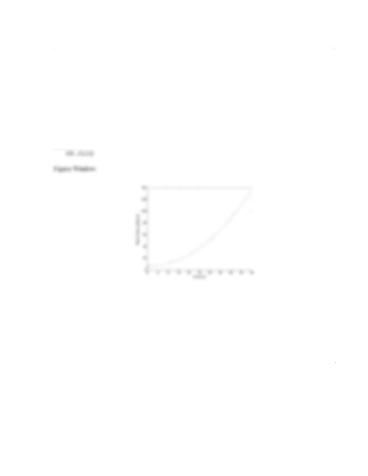
6.30 In a uniaxial tension test, a dog-bone-shaped specimen is pulled in a machine. During the test, the

force applied to the specimen, F, and the length of a gage section, L, are measured. The true stress, , and

the true strain, , are defined by:

and

where and are the initial cross-sectional area and gage length, respectively. The true stress–strain

curve in the region beyond the yield stress is often modeled by:

The following are values of F and L measured in an experiment. Use the approach from Section 6.3 for

determining the values of the coefficients K and m that best fit the data. The initial cross-sectional area and

gage length are m2, and m.

Solution

To solve the problem the equation is written in the form:

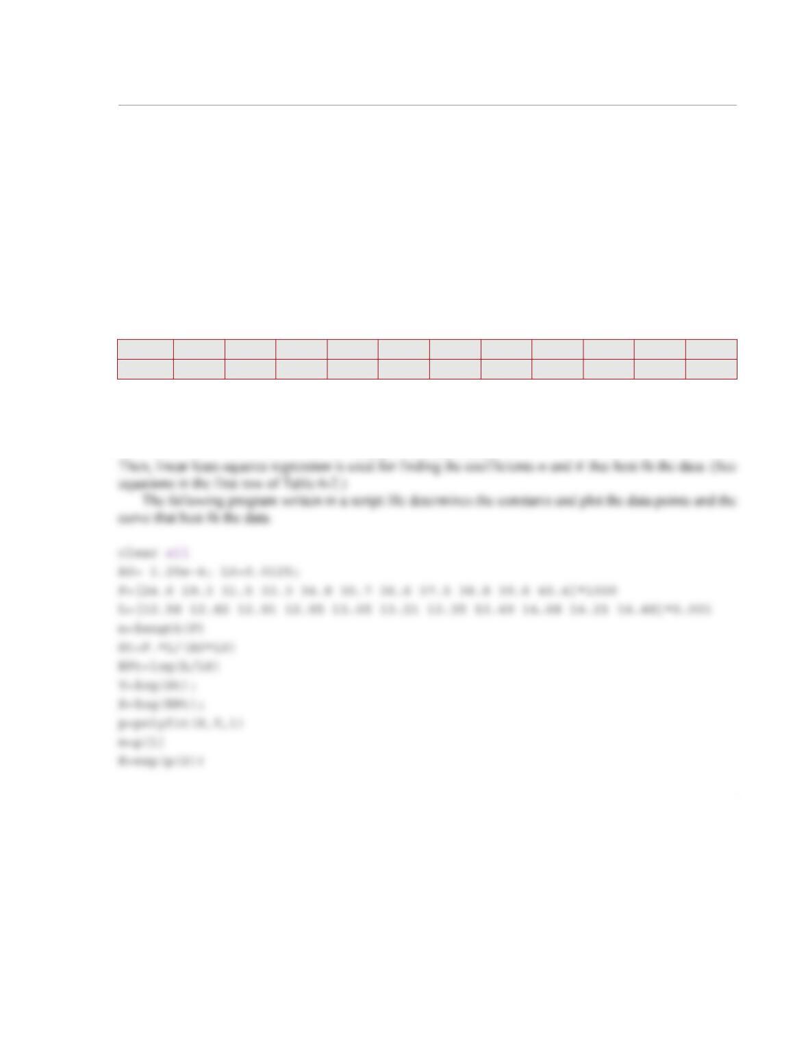
F (kN) 24.6 29.3 31.5 33.3 34.8 35.7 36.6 37.5 38.8 39.6 40.4

L (mm) 12.58 12.82 12.91 12.95 13.05 13.21 13.35 13.49 14.08 14.21 14.48

σt

εt

σt

F

A0

—– L

L0

—-–

=

εt

L

L0

—-–ln=

A0

L0

σtKεt

m

=

A01.25 10 4–

×=

L00.0125=

σtKεt

m

=

σt

()ln mεt

()ln K()ln+=

2

When the program is executed, the following values of m and K are displayed in the Command Window,

and the figure that follows is displayed in the Figure Window.

m =

0.2085

K =

5.4948e+008

1

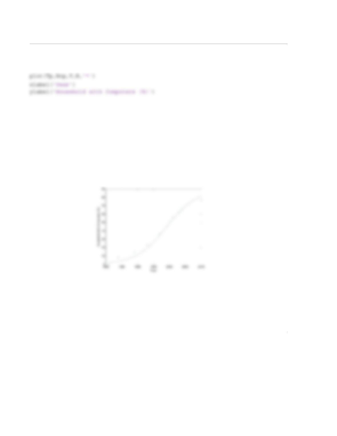
6.31 The percent of households that own at le ast one computer in selected years from 1981 to 2010,

according to the U.S. census bureau, is listed in the following table:

The data can be modeled with a function in the form (logistic equation), where

is percent of households that own at least one computer, C is a maximum value for , A and B are con-

stants, and x is the number of years after 1981. By using the method described in Section 6.3 and assuming

that , determine the constants A and B such that the function best fit the data. Use the function to

estimate the percent of ownership in 2008 and in 2013. In one figure, plot the function and the data points.

Solution

Rewriting the equation:

or

Year 1981 1984 1989 1993 1997 2000 2001 2003 2004 2010

Household with computer [%] 0.5 8.2 15 22.9 36.6 51 56.3 61.8 65 76.7

HCC1Ae Bx–

+()⁄=

HC

C90=

C

HC

——–1– Ae Bx–

=

C

HC

——–1–





ln Bx–Aln+=

2

Tp=1981:0.5:2010;

Hcp=Hc(Tp);

When the script is executed the following results are displayed in the Command Window, and the follow-

ing figure is displayed.

B =

0.2084

A =

9.5718e+180

Hc2008 =

77.5804