Keyton: Communication Research, 5e IM–1
Chapter 10
Testing for Differences
Activity: Determining Expected Cell Frequencies for Contingency Tables
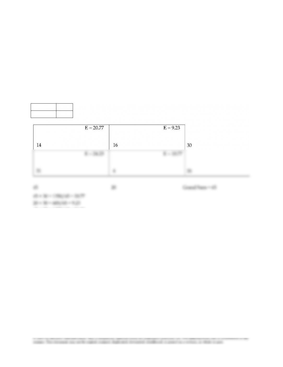
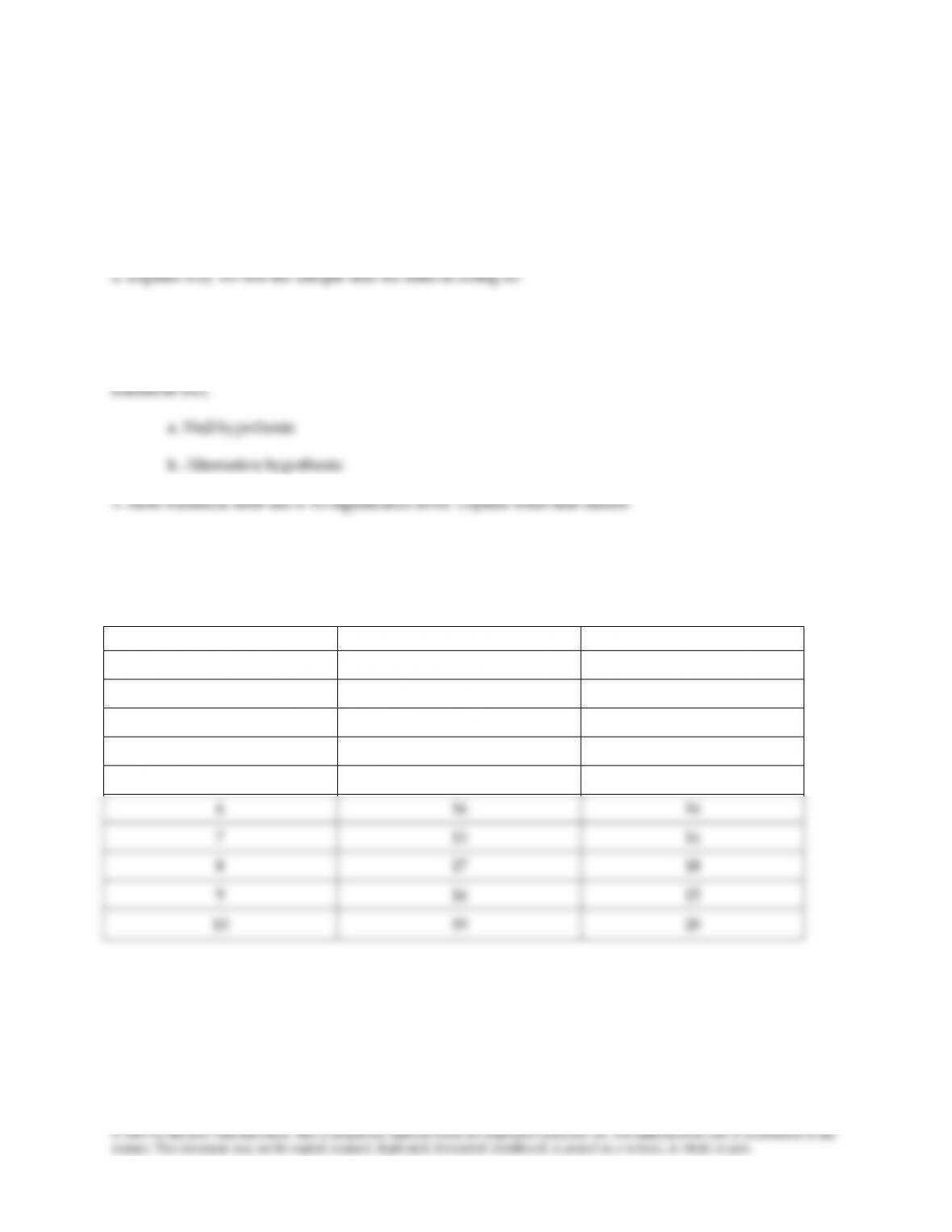
Ask students to use the data in the contingency table below to determine the expected frequencies for
each cell.
14
16
31
4
45 × 35 = 1575/65 = 24.23
20 × 35 = 700/65 = 10.77
Keyton: Communication Research, 5e IM–2
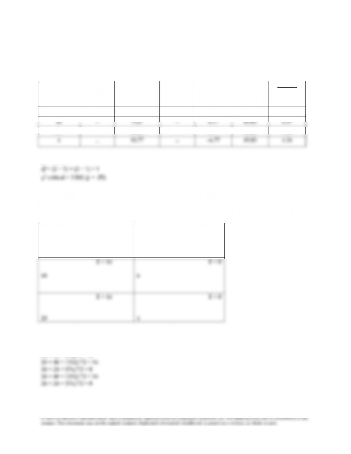
Activity: Computing 2
Ask students to compute 2 and interpret the result for the contingency table in the preceding activity.
See steps for contingency analysis in Appendix B (text, pages 360-361).
Observed
Frequency
(O)
Minus
Expected
Frequency (E)
Equals
(O – E)
(O – E)2
(O – E)2
E
14
–
20.77
=
–6.77
45.83
2.21
16
–
9.23
=
6.77
45.83
4.97
31
–
24.23
=
6.77
45.83
1.89
4
–
10.77
=
–6.77
45.83
4.26
2 = 13.33
Interpretation: The 2 of 13.33 exceeds 2 critical; support is provided for the research hypothesis.
Additional Data Set
10
E = 16
14
E = 8
18
E = 16
6
E = 8
20
E = 16
4
E = 8
48 24 Grand Sum = 72
24 × 48 = 1152/72 = 16
24 × 24 = 576/72 = 8
Keyton: Communication Research, 5e IM–3
Observed
Frequency
(O)
Minus
Expected
Frequency (E)
Equals
(O – E)
(O – E)2
(O – E)2
E
10
–
16
=
–6
36
2.25
14
–
8
=
6
36
4.50
18
–
16
=
2
4
0.25
6
–
8
=
–2
4
0.50
20
–
16
=
4
16
1
4
–
8
=
–4
16
2
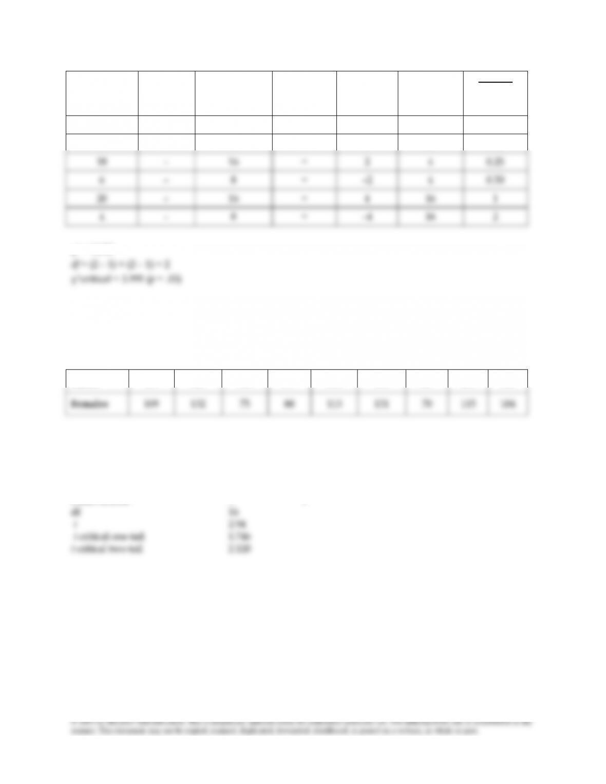
2 = 10.50
Activity: Significant Independent Sample t-Test
Ask students to compute t, evaluate the statistical significance of t, and interpret the result using the data
shown below. Change the variables as appropriate for your class, and create the corresponding
hypothesis to be tested.
Males
103
126
126
137
165
165
129
200
148
Females
109
132
75
88
113
151
70
115
104
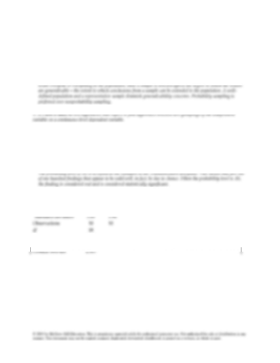
Results
Males Females
Mean 144.33 106.33
Standard deviation 28.80 26.04
Observations 9 9
Keyton: Communication Research, 5e IM–4
Additional Data Set
Communication majors
29
25
37
37
34
28
29
35
35
36
30
28
32
29
30
27
33
35
30
31
28
27
22
33
32
36
32
27
32
39
Nonmajors
24
21
28
22
20
20
24
15
26
13
27
29
22
26
26
26
21
22
19
22
18
17
16
20
29
24
23
19
19
26
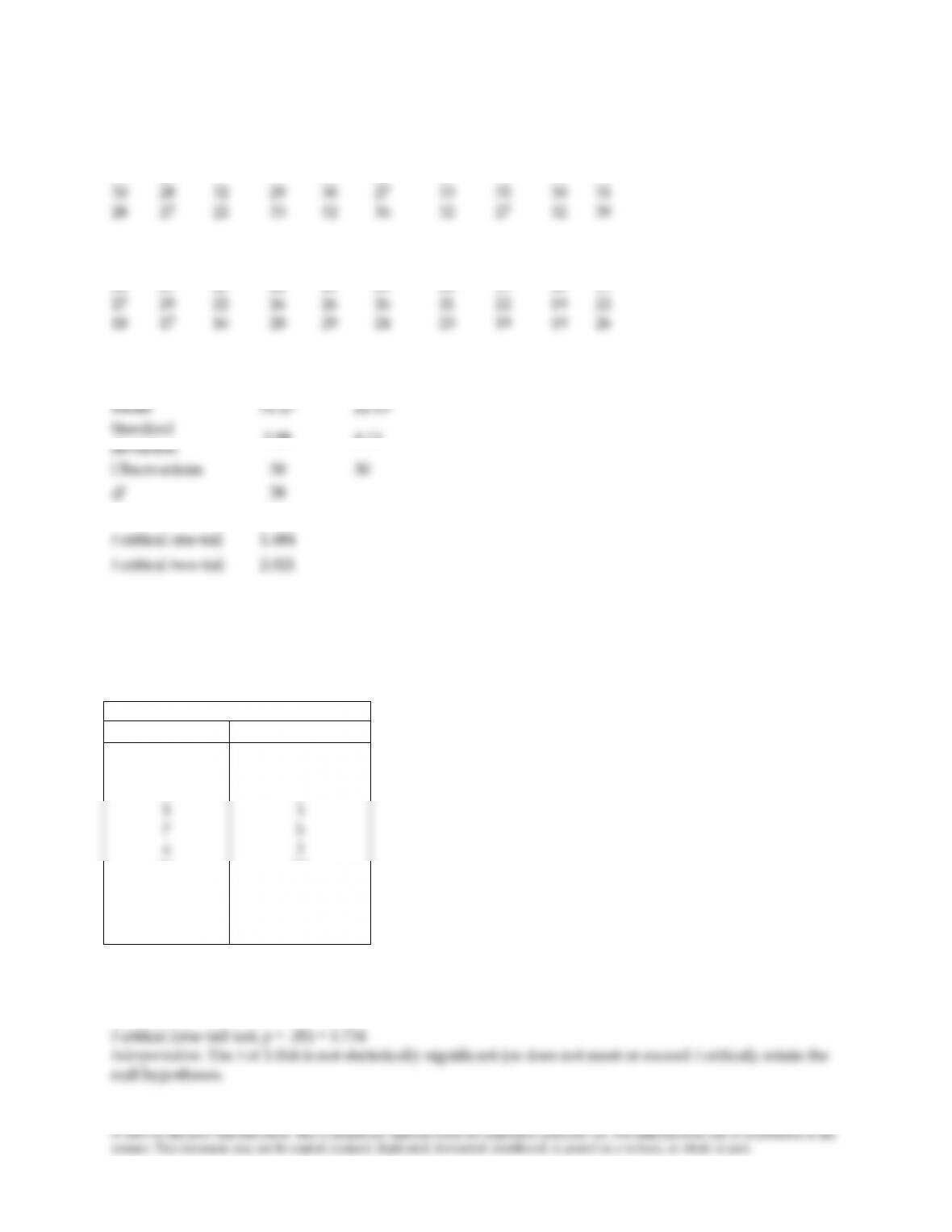
Results
Majors
Nonmajors
Mean
31.27
22.13
Standard
deviation
3.98
4.15
Observations
30
30
df
58
t
8.70
t critical one-tail
1.684
t critical two-tail
2.021
Activity: Nonsignificant Independent Sample t-Test
Ask students to compute t, evaluate the statistical significance of t, and interpret the result using the data
shown below. Change the variables as appropriate for your class, and create the corresponding
hypothesis to be tested.
Score on Leadership Effectiveness
Male
Female
4
12
6
5
7
4
16
5
9
10
3
9
8
3
5
2
10
6
8
8
Results
t = 1.044
df = (10 – 1) + (10 – 1) = 18
Keyton: Communication Research, 5e IM–5
Additional Data Sets
Trained
154
109
137
115
152
140
154
178
101
Untrained
103
126
126
137
165
126
129
200
148
Results
Trained
Untrained
Mean
137.78
140
Standard deviation
25.13
28.23
Observations
9
9
df (9 – 1) + (9 – 1)
16
t
–0.17639
t critical one-tail
1.745884
t critical two-tail
2.119905
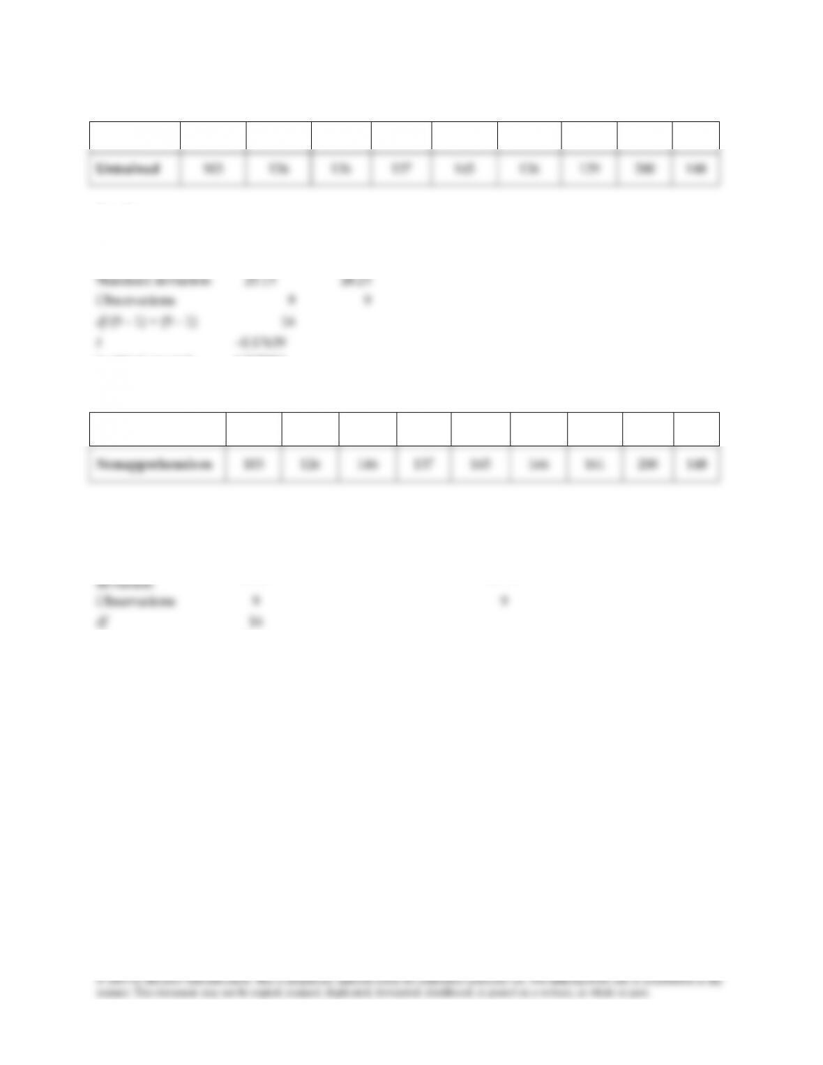
Apprehensives
154
109
137
115
152
140
154
178
101
Nonapprehensives
103
126
146
137
165
166
161
200
148
Results
Apprehensives Nonapprehensives
Mean
137.78
150.22
Standard
deviation
25.13
27.56
Observations
9
9
df
16
t
–1.00104
t critical one-tail
1.746
t critical two-tail
2.120
Keyton: Communication Research, 5e IM–6
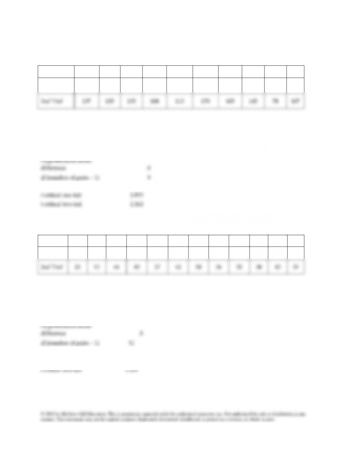
Activity: Paired Comparison t-Test
Develop a data scenario and context for your students. Ask them to compute a paired comparison t-test
using the data shown below.
Subject
1
2
3
4
5
6
7
8
9
10
1st Trial
113
105
130
101
138
118
87
116
75
96
2nd Trial
137
105
133
108
115
170
103
145
78
107
Results
1st Trial
2nd Trial
Mean
107.9
120.1
Observations
10
10
Hypothesized mean
difference
0
df (number of pairs – 1)
9
t
–1.92749
t critical one-tail
1.833
t critical two-tail
2.262
Additional Data Sets
Subject
1
2
3
4
5
6
7
8
9
10
11
12
1st Trial
24
23
47
42
26
46
38
33
28
28
21
27
2nd Trial
25
13
44
45
57
42
50
36
35
38
43
31
Results
1st Trial
2nd Trial
Mean
31.92
38.25
Observations
12
12
Hypothesized mean
difference
0
df (number of pairs – 1)
11
t
–1.93324
t critical one-tail
1.796
t critical two-tail
2.201
Keyton: Communication Research, 5e IM–7
Stats Worksheet—Chi-Square
2. There are two types of chi-squares. Identify each and give an example.
4. Cell size can be problematic with chi-square. Describe the problem.
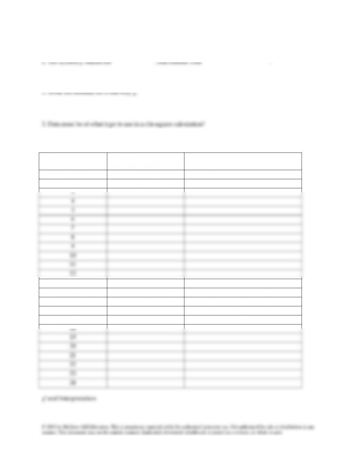
6. From the data we collect in class on the form below, compute the chi-square. Interpret your findings.
Subject Number
Sex
Female, Male
Year in School
Freshman, Sophomore, Junior, Senior
1
2
3
4
5
6
7
8
9
10
11
12
13
14
15
16
17
18
19
20
21
22
23
24
Keyton: Communication Research, 5e IM–8
Answer Key for Stats Worksheet—Chi-Square
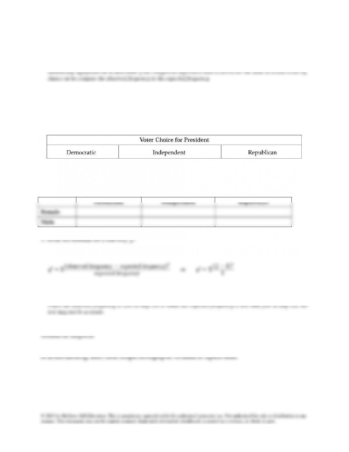
1. The symbol 2 stands for chi-square. This statistic tests to determine if differences among categories are
2. There are two types of chi-squares. Identify each and give an example.
a. One-way chi-square. Used to determine if differences in how the cases are distributed across the categories of
one categorical or nominal variable are significant.
Example: Did you vote for the Democratic, Independent, or Republican candidate for president?
b. Contingency analysis. Tests to see how frequencies for one variable are contingent on, or relative to, frequencies
for the other variable.
Example: How did voter sex differ with respect to voting choice for the Democratic, Independent, or
Republican candidate for president?
Democratic
Independent
Republican
Female
Male
4. Cell size can be problematic with chi-square. Describe the problem.
5. Data must be of what type to use in a chi–square calculation?
6. Note: Use the form to collect data from students in class. If your class is not varied with respect to sex
Keyton: Communication Research, 5e IM–9
Stats Worksheet—t-Test
1. A population is
A sample is
3. A t-test is used to
4. Using males and females as levels for the independent variable and communication competence scores
as the dependent variable, write a null hypothesis and an alternative hypothesis using t-test as the
6. Husbands and wives were compared for their level of satisfaction with their marital interaction. Their
scores are shown below. Using a t–test as the statistical tool, write a null hypothesis and an alternative
hypothesis for this example. Compute the t-test and compare it with t critical. Interpret your findings.
Couple #
Husbands
Wives
1
19
16
2
24
22
3
21
20
4
23
15
5
14
13
6
16
16
7
15
14
8
17
18
9
16
15
10
19
20
Keyton: Communication Research, 5e IM–10
Answer Key for Stats Worksheet—t-Test
1. A population is all units or the universe—people or things—possessing the attributes or characteristics in
which the researcher is interested. A sample is a subset, or portion, of a population.
2. Explain why we test the sample and the risks in doing so.
Generally, it is impossible, impractical, or both, to ask everyone to participate in a research project or to even
4. a. Null hypothesis: There will be no difference in communication competence scores for males and females.
b. Alternative hypothesis: (Example) Females will have higher communication competence scores than males.
5. Most statistical tests use a .05 significance level. Explain what that means.
6. Results
Husbands
Wives
Mean
18.4
16.9
Standard deviation
3.41
2.96
Observations
10
10
df
18
t
1.051
t critical one-tail
1.734
t critical two-tail
2.101
Keyton: Communication Research, 5e IM–11
Stats Worksheet—ANOVA
1. a. ANOVA stands for ________________________________________, a statistical test that
___________________________________________________________________________________. More
specifically, an ANOVA tests to see if the variance _______________ is greater than the variance
_______________. The statistical symbol used for ANOVA is _______________.
b. The independent variable(s) must be of what type of data?
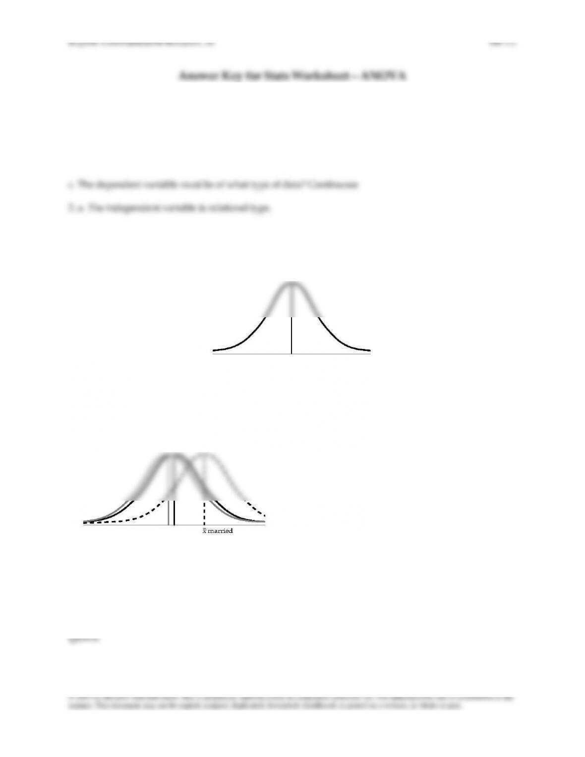
c. The dependent variable must be of what type of data?
2. The purpose of a study is to compare relational satisfaction for three types of people: (a) married, (b)
living together, but not married, or (c) just dating, not living together. Write a null hypothesis and an
alternative hypothesis using ANOVA as your statistic. Demonstrate the presumed outcome for the
3. A two-way ANOVA is when there are two _______________ variables. When there are two or more
variables, we can also test for the _______________ effect. If the interaction is significant, how do we
interpret the main effects?
4. In ANOVAs, there can be only one _____________ variable.
6. A 2 × 3 × 4 ANOVA means that
Keyton: Communication Research, 5e IM–13
6. A 2 × 3 × 4 ANOVA means that the ANOVA is three way or has three independent variables. The first
independent variable has two levels, the second variable has three levels, and the third variable has four levels.
Additional Resources
Hayes, J. G., & Metts, S. (2008). Managing the expression of emotion. Western Journal of Communication, 72,
374-396. doi:10.1080/10570310802446031
Gilchrist, E. (2010). A sweet approach to teaching the one-variable chi-square test. Communication Teacher,
24, 13-17. doi:10.1080/17404620903433424
Professor Gilchrist describes an interesting in-class activity to help students learn chi-squares. Using
candy (Skittles or M&Ms), students calculate the observed frequency of candy colors with the expected
frequencies of candy colors [yes, there is an expected frequency according to Mars Incorporated]. As she
reports, the activity helps student learn the statistical procedure and provides a motivating treat.
There are many statistics sites, but few are really free. Here is one that covers ANOVA:
http://www.statisticshowto.com/probability-and-statistics/hypothesis-testing/anova/#ANOVA
Web Resources
For a list of Internet resources, visit https://www.joannkeyton.com/research-methods