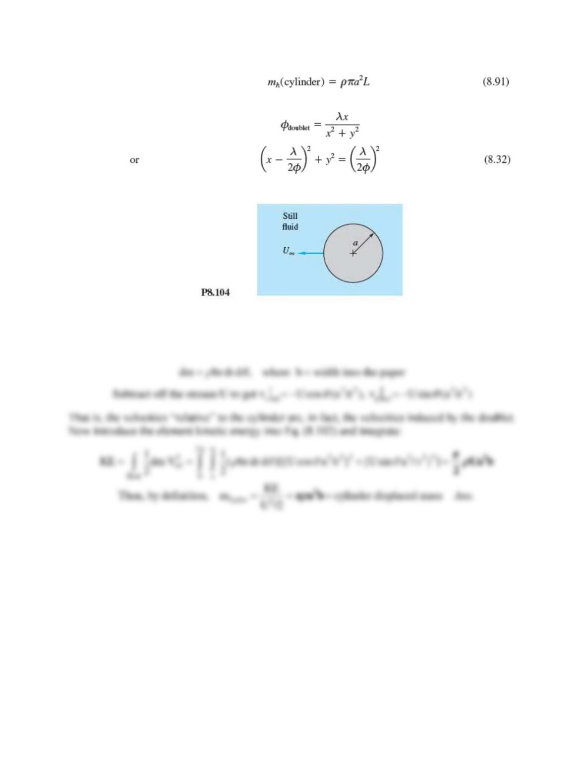
Solution 8.104
For this two-dimensional polar-coordinate system, a differential mass is:
Problem 8.105
A 22-cm-diameter solid aluminum sphere (SG = 2.7) is accelerating at 12 m/s2 in water at 20C.
(a) According to potential theory, what is the hydrodynamic mass of the sphere? (b) Estimate
the force being applied to the sphere at this instant.
Solution 8.105
For water at 20C, take
= 998 kg/m3. The sphere radius is a = 11 cm. (a) Equation (8.103)
gives the hydrodynamic mass, which is proportional to the water density:
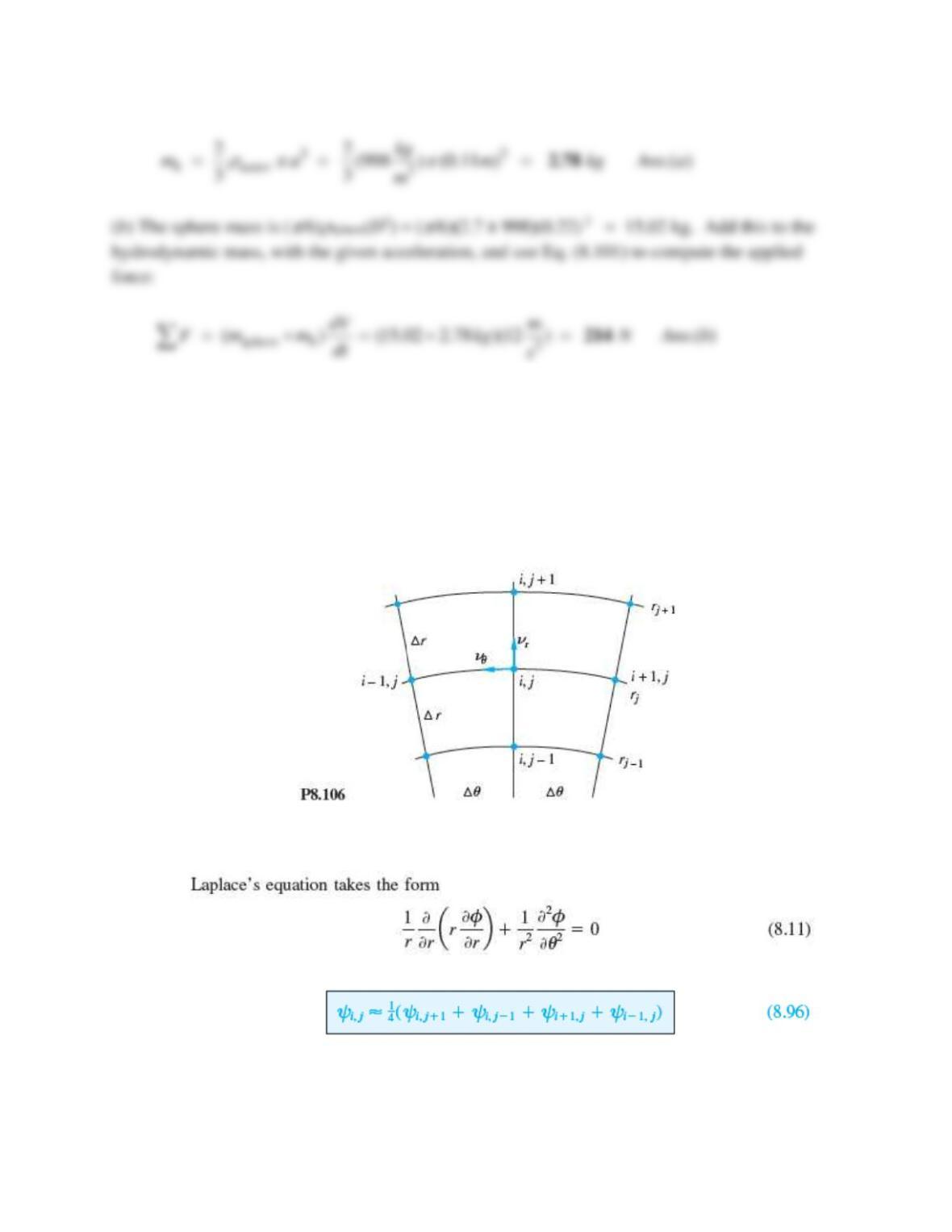
Problem 8.106
Laplace’s equation in plane polar co-ordinates, Eq. (8.11), is complicated by the variable radius.
Consider the finite-difference mesh in Fig. P8.106, with nodes (i, j) at equally spaced
and r.
Derive a finite-difference model for Eq. (8.11) similar to our cartesian expression in Eq. (8.96).
Solution 8.106
We are asked to model
Problem 8.107
SAE 10W30 oil at 20ºC is at rest near a wall when the wall suddenly begins moving at a constant
1 m/s. (a) Use Δy = 1 cm and Δt = 0.2 s and check the stability criterion (8.101). (b) Carry out
Eq. (8.100) to t = 2 s and report the velocity u at y = 4 cm.
Solution 8.107
From Table A.3 for SAE 10W30 oil, ρ= 876 kg/m3 and μ = 0.17 kg/m∙s. Then
2
22 OK
0.17 (0.000194)(0.2)
0.000194 ; 0.388 0.5
876 ( ) (0.01)
mt
sy
= = = = = =
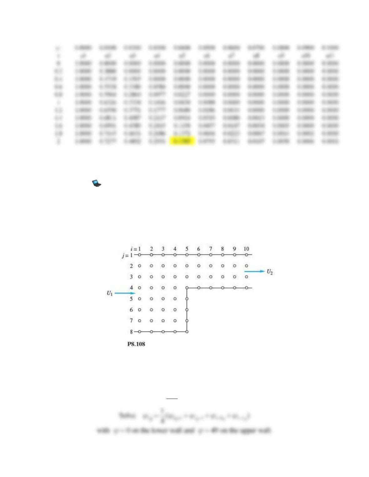
The predicted velocity at 2 s and 4 cm is 0.1585 m/s. The exact solution [15, p. 130] is
0.1511 m/s.
Problem 8.108
Consider two-dimensional potential flow into a step contraction as in Fig. P8.108. The inlet
velocity U1 = 7 m/s, and the outlet velocity U2 is uniform. The nodes (i, j) are labeled in the
figure. Set up the complete finite-difference algebraic relation for all nodes. Solve, if possible, on
a computer and plot the streamlines in the flow.
Solution 8.108
By continuity, U2 = U1(7/3) = 16.33 m/s. For a square mesh, the standard Laplace model,
Eq. (8.109), holds. For simplicity, assume unit mesh widths x = y = 1.
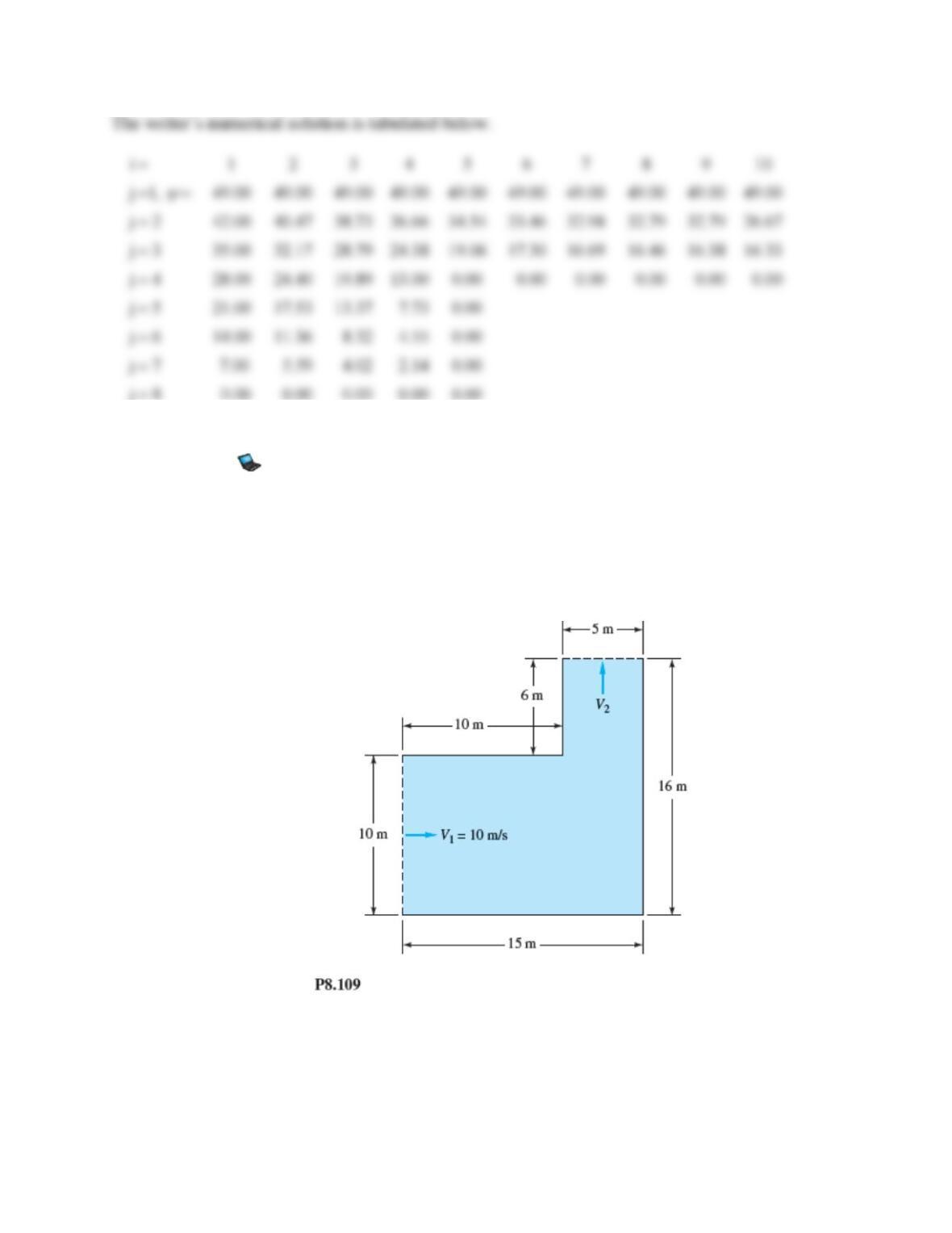
Problem 8.109
Consider inviscid potential flow through a two-dimensional 90 bend with a contraction, as in
Fig. P8.109. Assume uniform flow at the entrance and exit. Make a finite-difference computer
analysis for small grid size (at least 150 nodes), determine the dimensionless pressure
distribution along the walls, and sketch the streamlines. (You may use either square or
rectangular grids.)
Solution 8.109
This problem is “digital computer enrichment” and will not be presented here.
Problem 8.110
For fully developed laminar incompressible flow through a straight noncircular duct, as in Sec.
6.8, the Navier-Stokes Equation (4.38) reduce to
22
22
1const 0
u u dp
dx
yz
+ = =
where (y, z) is the plane of the duct cross section and x is along the duct axis. Gravity is
neglected. Using a nonsquare rectangular grid (x, y), develop a finite-difference model for this
equation, and indicate how it may be applied to solve for flow in a rectangular duct of side
lengths a and b.
Solution 8.110
An appropriate square grid is shown above. The finite-difference model is
Problem 8.111
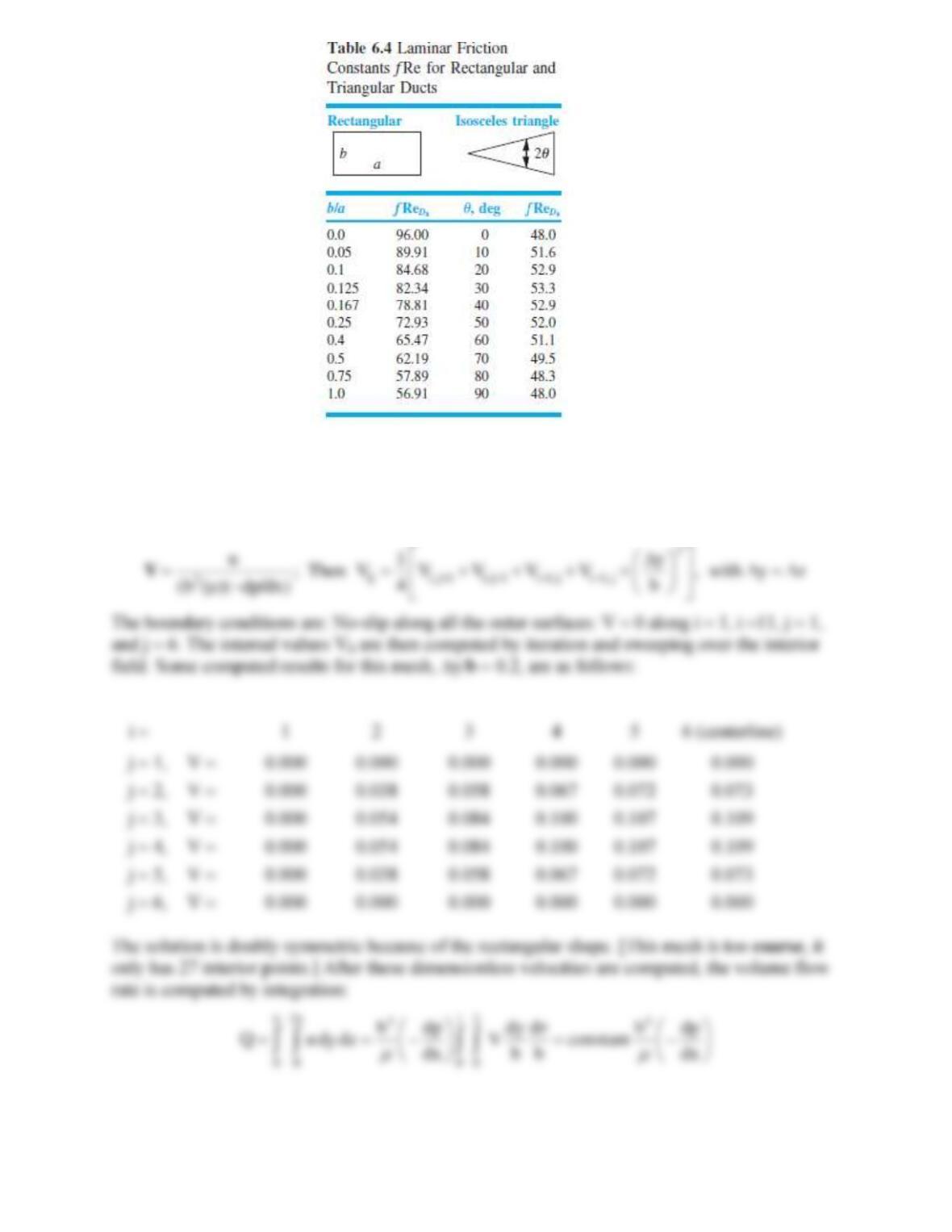
Solve Prob. 8.110 numerically for a rectangular duct of side length b by 2b, using at least
100 nodal points. Evaluate the volume flow rate and the friction factor, and compare with the
results in Table 6.4:
4
0.1143 Re 62.19
h
D
b dp
Qf
dx
−
where Dh = 4A/P = 4b/3 for this case. Comment on the possible truncation errors of your model.
Solution 8.111
A typical square mesh is shown in the figure above. It is appropriate to nondimensionalize the
velocity and thus get the following dimensionless model:
Problem 8.112
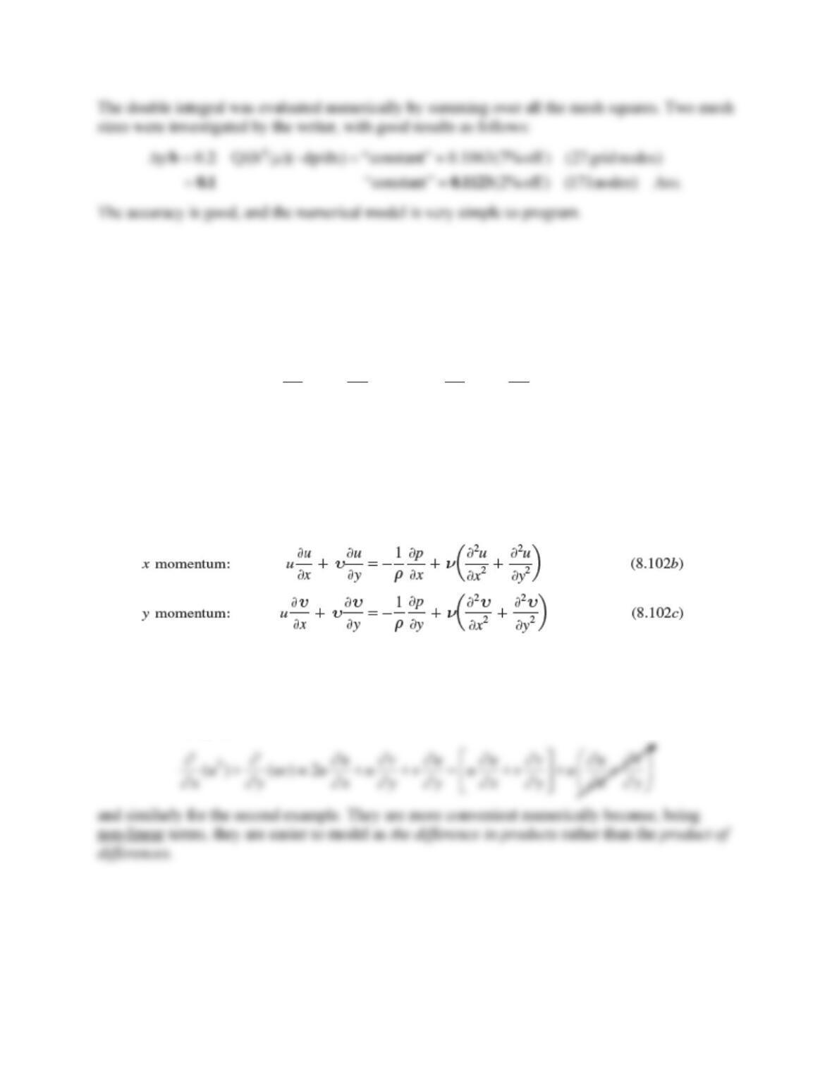
In CFD textbooks [5, 23-27], one often replaces the left-hand side of Eq. (8.102b and c),
respectively, with the following two expressions:
22
( ) ( ) and ( ) ( ) u vu uv v
x y x y
++
Are these equivalent expressions, or are they merely simplified approximations? Either way, why
might these forms be better for finite-difference purposes?
Solution 8.112
These expressions are indeed equivalent because of the 2-D incompressible continuity equation.
In the first example,
Problem 8.113
Formulate a numerical model for Eq. (8.99), which has no instability, by evaluating the second
derivative at the next time step, j+1. Solve for the center velocity at the next time step and
comment on the result. This is called an implicit model and requires iteration.
Solution 8.113
This new finite difference model would be as follows:
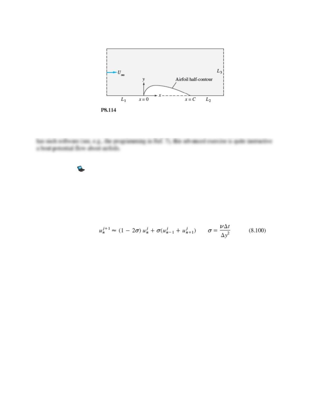
Problem 8.114
If your institution has an online potential flow boundary-element computer code, consider
flow past a symmetric airfoil, as in Fig. P8.114. The basic shape of an NACA symmetric airfoil
is defined by the function [12]
1/2 2
max
34
21.4845 0.63 1.758
1.4215 0.5075
y
t
− −
+−
where
= x/C and the maximum thickness tmax occurs at
= 0.3. Use this shape as part of the
lower boundary for zero angle of attack. Let the thickness be fairly large, say, tmax = 0.12, 0.15, or
0.18. Choose a generous number of nodes (60), and calculate and plot the velocity distribution
V/U along the airfoil surface. Compare with the theoretical results in Ref. 12 for NACA 0012,
0015, or 0018 airfoils. If time permits, investigate the effect of the boundary lengths L1, L2, and
L3, which can initially be set equal to the chord length C.
Solution 8.114*
This problem is not solved here. It requires Boundary-Element-Code software. If your institution
Problem 8.115
Use the explicit method of Eq. (8.100) to solve Problem 4.85 numerically for SAE 30 oil with
Uo = 1 m/s and
= M rad/s, where M is the number of letters in your surname. (The writer will
solve it for M = 5.) When steady oscillation is reached, plot the oil velocity versus time at
y = 2 cm.
Problem 4.85
A flat plate of essentially infinite width and breadth oscillates sinusoidally in its own plane beneath a
viscous fluid, as in Fig. P4.85. The fluid is at rest far above the plate. Making as many simplifying
assumptions as you can, set up the governing differential equation and boundary conditions for
finding the velocity field u in the fluid. Do not solve (if you can solve it immediately, you might be
able to get exempted from the balance of this course with credit).
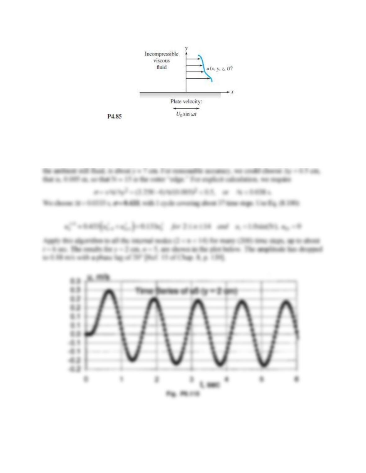
Solution 8.115
Recall that Prob. 4.85 specified an oscillating wall, uwall = Uosin(
t). One would have to
experiment to find that the “edge” of the shear layer, that is, where the wall no longer influences