Problem 8.C1
Did you know that you can solve simple fluid mechanics problems with Microsoft Excel? The
successive relaxation technique for solving the Laplace equation for potential flow problems is
easily set up on a spreadsheet, since the stream function at each interior cell is simply the average
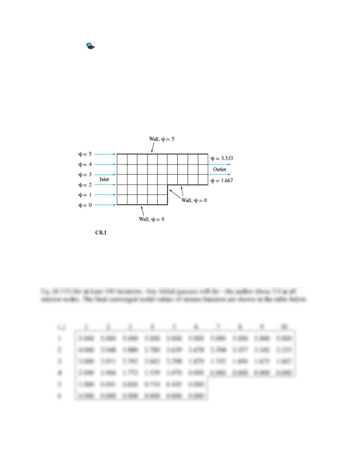
of its four neighbors. As an example, solve for the irrotational potential flow through a
contraction, as given in Fig. C8.1. Note: To avoid the “circular reference” error, you must turn
on the iteration option. Use the help index for more information. For full credit, attach a printout
of your spreadsheet, with stream function converged and the value of the stream function at each
node displayed to four digits of accuracy.
Solution 8.C1
Do exactly what the figure shows: Set bottom nodes at
= 0, top nodes at
= 5, left nodes at
= 0, 1, 2, 3, 4, 5 and right nodes at
= 0, 1.667, 3.333, and 5. Iterate with
Problem 8.C2
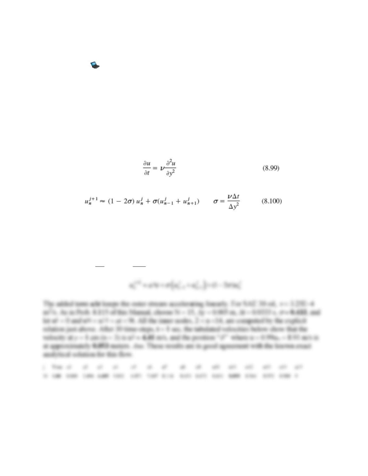
Use an explicit method, similar to but not identical to Eq. (8.100), to solve the case of SAE 30 oil
starting from rest near a fixed wall. Far from the wall, the oil accelerates linearly, that is,
u = uN = at, where a = 9 m/s2. At t = 1 s, determine (a) the oil velocity at y = 1 cm; and (b) the
instantaneous boundary layer thickness (where u 0.99u).
Hint: There is a non-zero pressure gradient in the outer (shear-free) stream, n = N, which must be
included in Eq. (8.99).
Solution 8.C2
To account for the stream acceleration as
2u/
t2 = 0, we add a term:
2
2
, which changes the model of Eq (8.100) to
uu
a.
ty
=+
Problem 8.C3
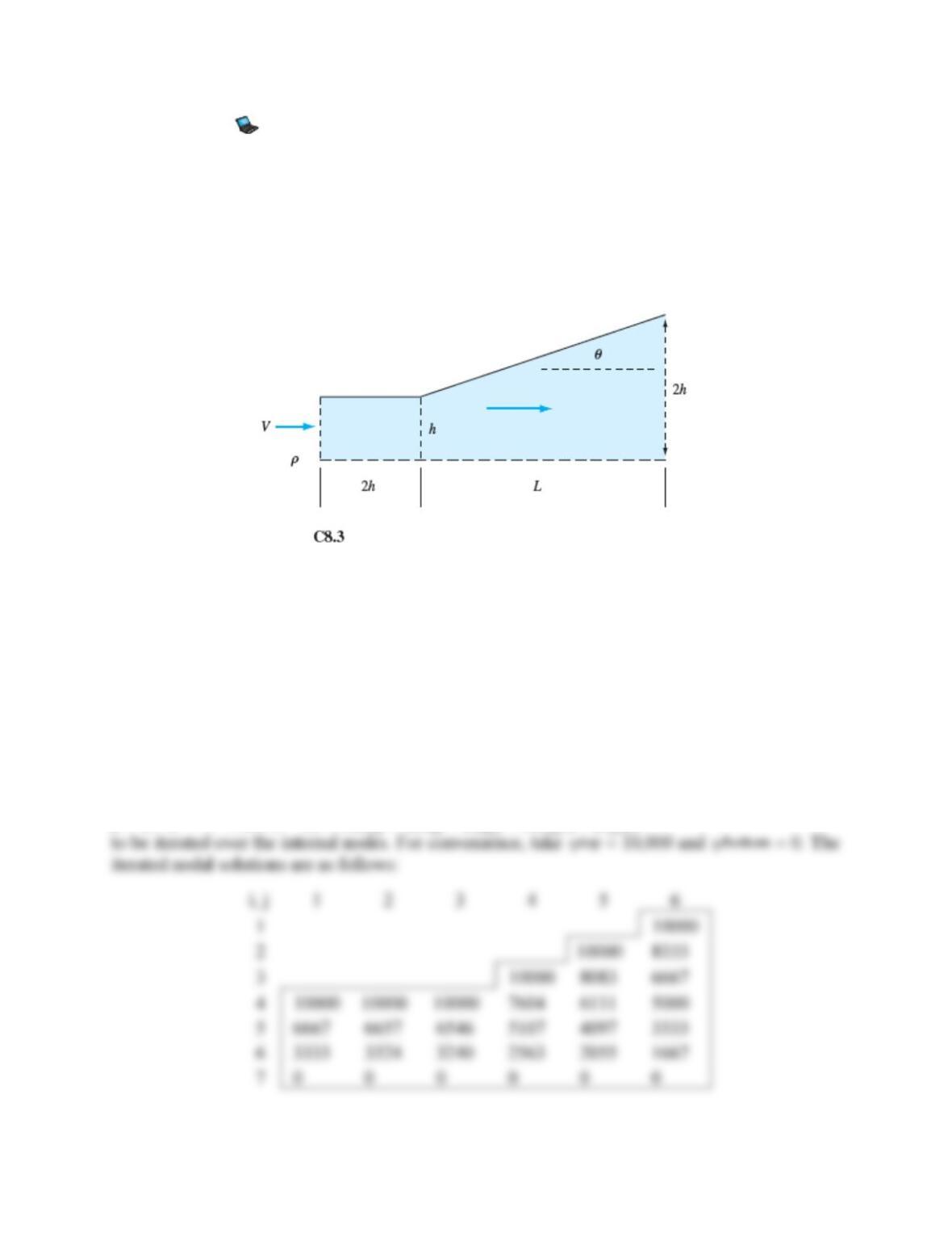
Consider plane inviscid flow through a symmetric diffuser, as in Fig. C8.3. Only the upper half is
shown. The flow is to expand from inlet half-width h to exit half-width 2h, as shown. The
expansion angle θ is 18.5° (L ≈ 3h). Set up a nonsquare potential flow mesh for this problem,
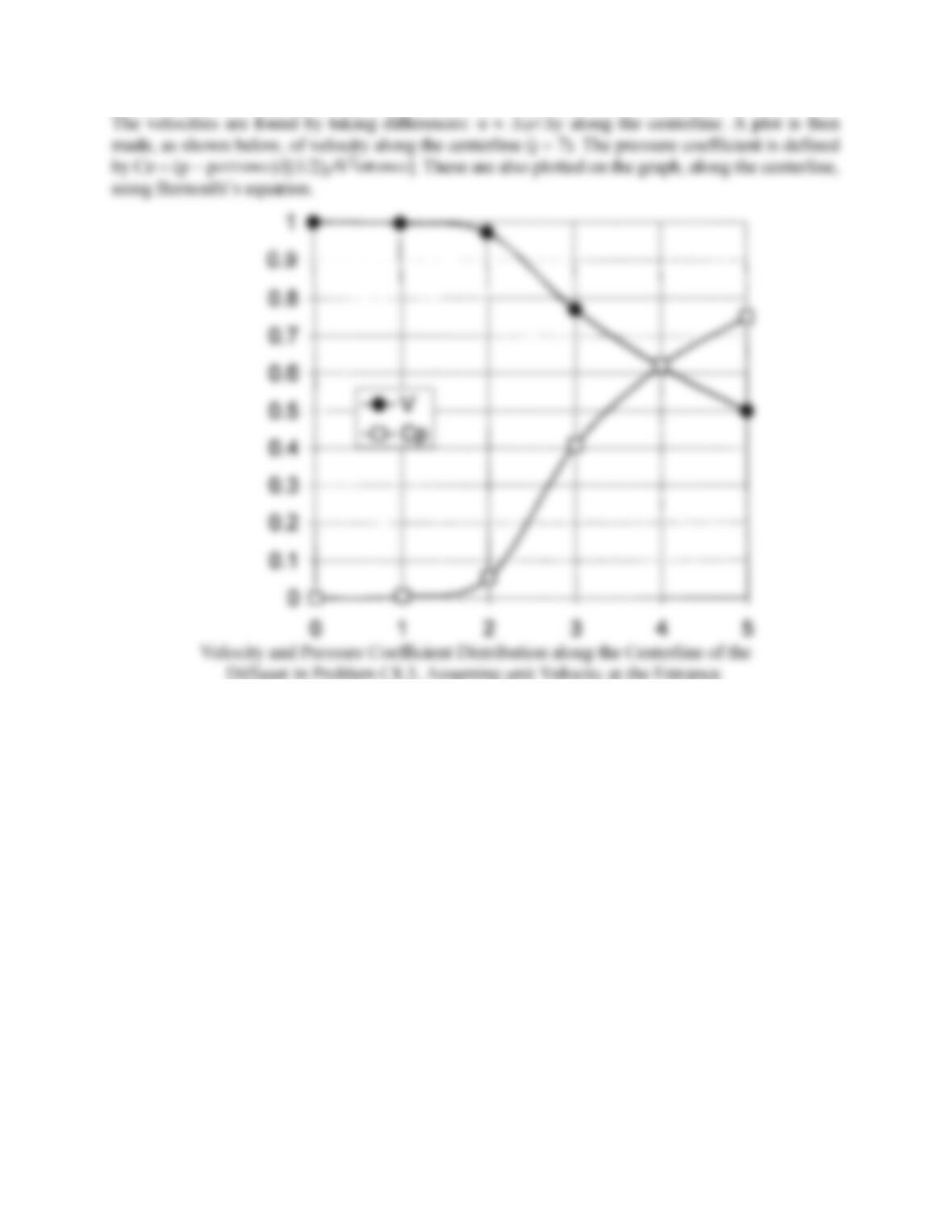
and calculate and plot (a) the velocity distribution and (b) the pressure coefficient along the
centerline. Assume uniform inlet and exit flows.
Solution 8.C3
The tangent of 18.5 is 0.334, so L 3h and 3:1 rectangles are appropriate. If we make them
h long and h/3 high, then i = 1 to 6 and j = 1 to 7. The model is given by Eq. (8.108) with
= (3/1)2 = 9. That is,
2(1 9) 9( )
+ + + +
Problem 8.C4
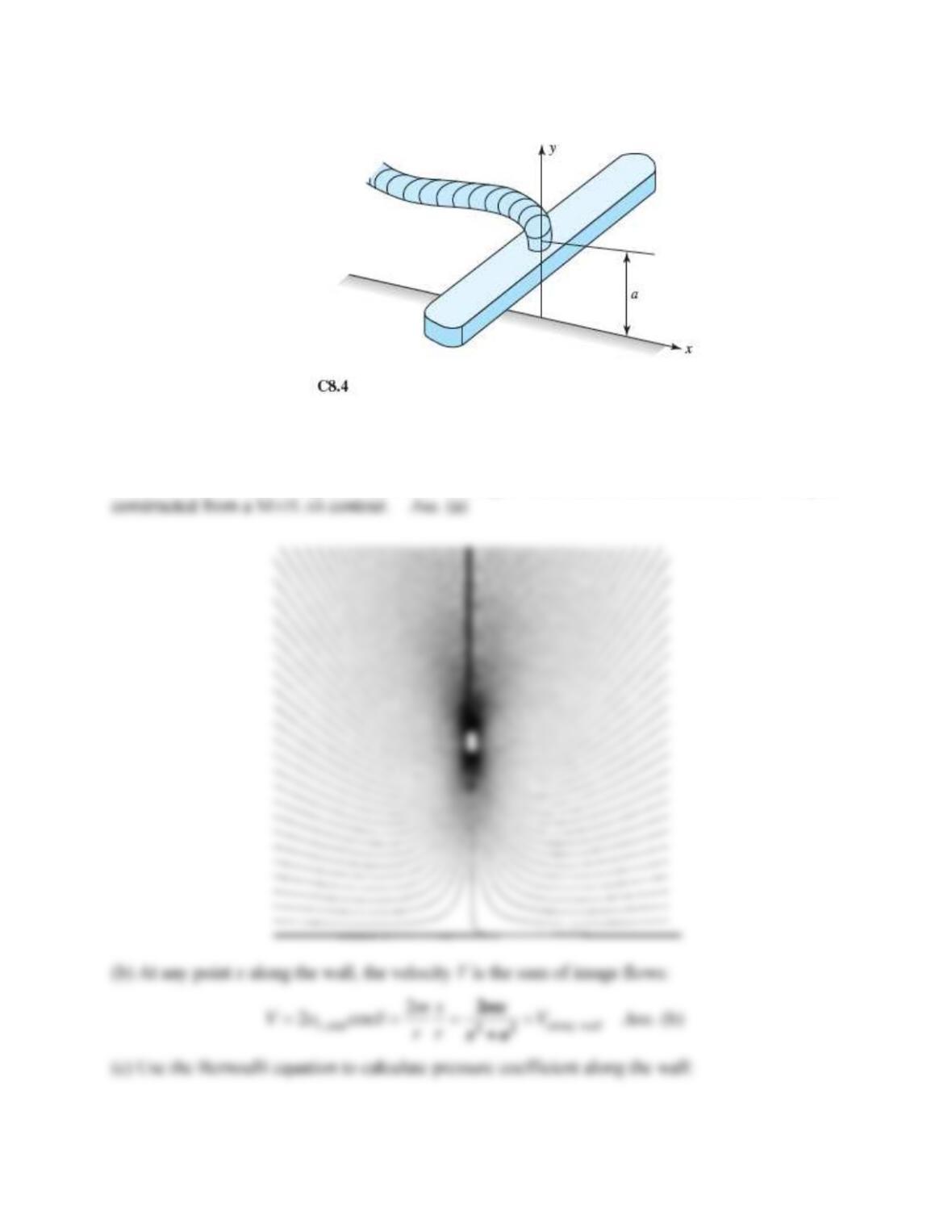
Use potential flow to approximate the flow of air being sucked up into a vacuum cleaner through
a two-dimensional slit attachment, as in Fig. C8.4. In the xy plane through the centerline of the
attachment, model the flow as a line sink of strength (2m), with its axis in the z direction at
height a above the floor. (a) Sketch the streamlines and locate any stagnation points in the flow.
(b) Find the magnitude of velocity V(x) along the floor in terms of the parameters a and m.
(c) Let the pressure far away be p∞, where velocity is zero. Define a velocity scale U = m/a.
Determine the variation of dimensionless pressure coefficient, Cp = (p − p∞)/(ρU2/2), along the
floor. (d) The vacuum cleaner is most effective where Cp is a minimum—that is, where velocity
is maximum. Find the locations of minimum pressure coefficient along the x axis. (e) At which
points along the x axis do you expect the vacuum cleaner to work most effectively? Is it best at
x = 0 directly beneath the slit, or at some other x location along the floor? Conduct a scientific
experiment at home with a vacuum cleaner and some small pieces of dust or dirt to test your
prediction. Report your results and discuss the agreement with prediction. Give reasons for any
disagreements.
Solution 8.C4
(a) The “floor” is created by a sink at (0, +a) and an image sink at (0, −a), exactly like Fig. 8.17a
of the text. There is one stagnation point, at the origin. The streamlines are shown below in a plot
Problem 8.C5
Consider a three-dimensional, incompressible, irrotational flow. Use the following two methods
to prove that the viscous term in the Navier-Stokes equation is identically zero: (a) using vector
notation; and (b) expanding out the scalar terms and substituting terms from the definition of
irrotationality.
Solution 8.C5
(a) For irrotational flow, V = 0, and V =
, so the viscous term may be rewritten in terms
of
and then we get Laplace’s equation:
Problem 8.C6
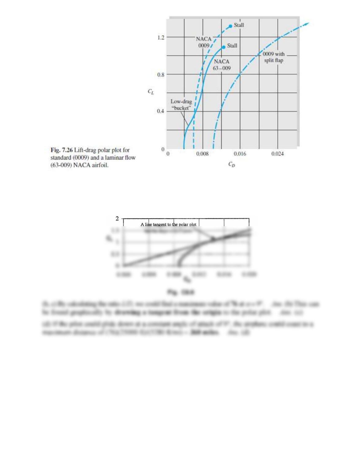
Find, either on-line or in Ref. 12, lift-drag data for the NACA 4412 airfoil. (a) Draw the polar
lift–drag plot and compare qualitatively with Fig. 7.26. (b) Find the maximum value of the lift-
to-drag ratio. (c) Demonstrate a straight-line construction on the polar plot that will immediately
yield the maximum L/D in (b). (d) If an aircraft could use this two-dimensional wing in actual
flight (no induced drag) and had a perfect pilot, estimate how far (in miles) this aircraft could
glide to a sea-level runway if it lost power at 25,000 ft altitude.
Solution 8.C6
(a) Simply calculate CL(
) and CD(
) and plot them versus each other, as shown below:
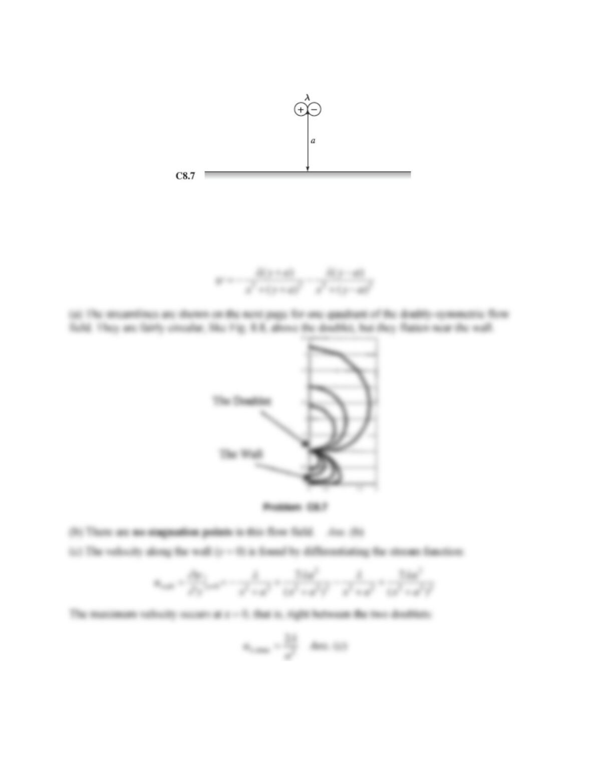
Problem 8.C7
Find a formula for the stream function for flow of a doublet of strength
at a distance a from a
wall, as in Fig. C8.7. (a) Sketch the streamlines. (b) Are there any stagnation points? (c) Find the
maximum velocity along the wall and its position.
Solution 8.C7
Use an image doublet of the same strength and orientation at the (x, y) = (0, −a). The stream function
for this combined flow will form a “wall” at y = 0 between the two doublets:
Problem 8.W1
What simplifications have been made, in the potential flow theory of this chapter, which result in
the elimination of the Reynolds number, Froude number, and Mach number as important
parameters?
Solution 8.W1
Problem 8.W2
In this chapter we superimpose many basic solutions, a concept associated with linear equations.
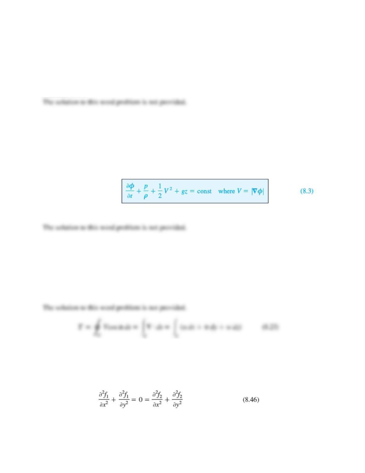
Yet Bernoulli’s equation (8.3) is nonlinear, being proportional to the square of the velocity. How,
then, do we justify the use of superposition in inviscid flow analysis?
Solution 8.W2
Problem 8.W3
Give a physical explanation of circulation Γ as it relates to the lift force on an immersed body. If
the line integral defined by Eq. (8.23) is zero, it means that the integrand is a perfect
differential—but of what variable?
Solution 8.W3
Problem 8.W4
Give a simple proof of Eq. (8.46)—namely, that both the real and imaginary parts of a function
f(z) are Laplacian if z = x + iy. What is the secret of this remarkable behavior?
Solution 8.W4
Problem 8.W5
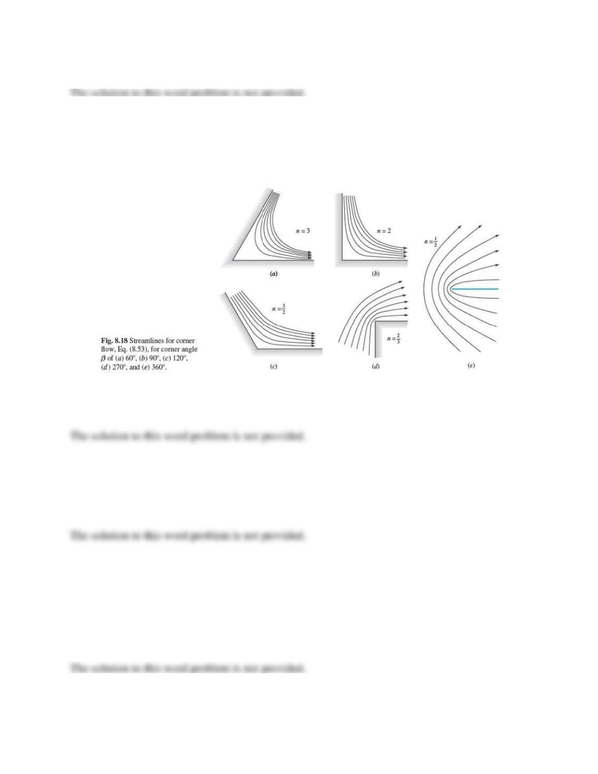
Figure 8.18 contains five body corners. Without carrying out any calculations, explain physically
what the value of the inviscid fluid velocity must be at each of these five corners. Is any flow
separation expected?
Solution 8.W5
Problem 8.W6
Explain the Kutta condition physically. Why is it necessary?
Solution 8.W6
Problem 8.W7
We have briefly outlined finite difference and boundary element methods for potential flow but
have neglected the finite element technique. Do some reading and write a brief essay on the use
of the finite element method for potential flow problems.
Solution 8.W7
Problem 8.1
Prove that the streamlines
(r,
) in polar coordinates, from Eq. (8.10), are orthogonal to the
potential lines
(r,
).
Solution 8.1
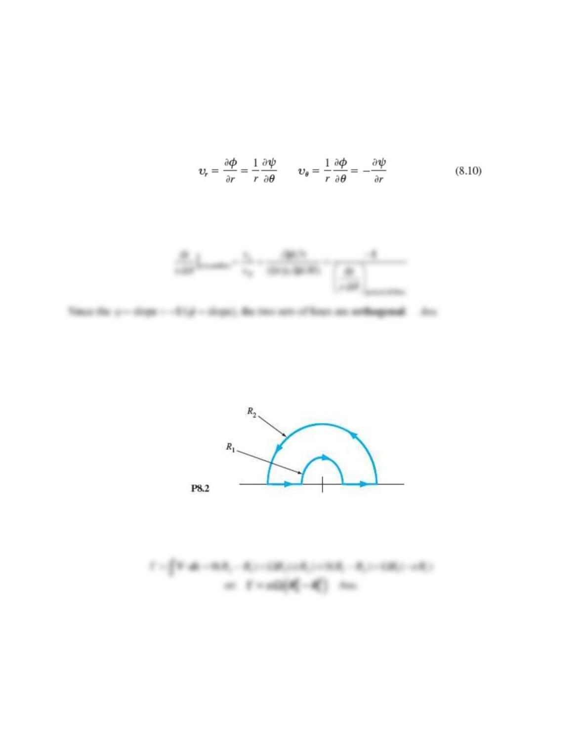
The streamline slope is represented by
Problem 8.2
The steady plane flow in Fig. P8.2 has the polar velocity components v
= r and vr = 0.
Determine the circulation around the path shown.
Solution 8.2
Start at the inside right corner, point A, and go around the complete path:
Problem 8.3
Using cartesian coordinates, show that each velocity component (u, v, w) of a potential flow
satisfies Laplace’s equation separately.
Solution 8.3
This is true because the order of integration may be changed in each case:
x x x
Problem 8.4
Is the function 1/r a legitimate velocity potential in plane polar coordinates? If so, what is the
associated stream function
( r,
) ?
Solution 8.4
Evaluation of the laplacian of (1/r) shows that it is not legitimate:
Problem 8.5
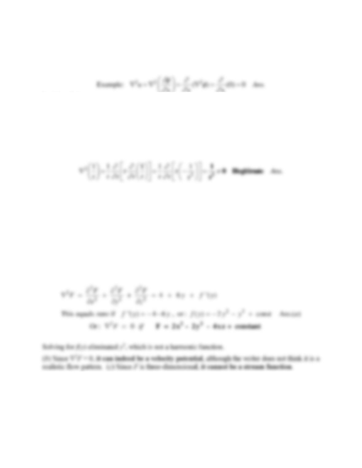
A proposed harmonic function F(x, y, z) is given by
23
2 4 ( )F x y x z f y= + − +
(a) If possible, find a function f(y) for which the Laplacian of F is zero. If you do indeed solve part (a),
can your final function F serve as (b) a velocity potential, or (c) a stream function?
Solution 8.5
Evaluate 2F and see if we can find a suitable f(y) to make it zero:
Problem 8.6
An incompressible plane flow has the velocity potential
= 2Bxy, where B is a constant. Find
the stream function of this flow, sketch a few streamlines, and interpret the flow pattern.
Solution 8.6
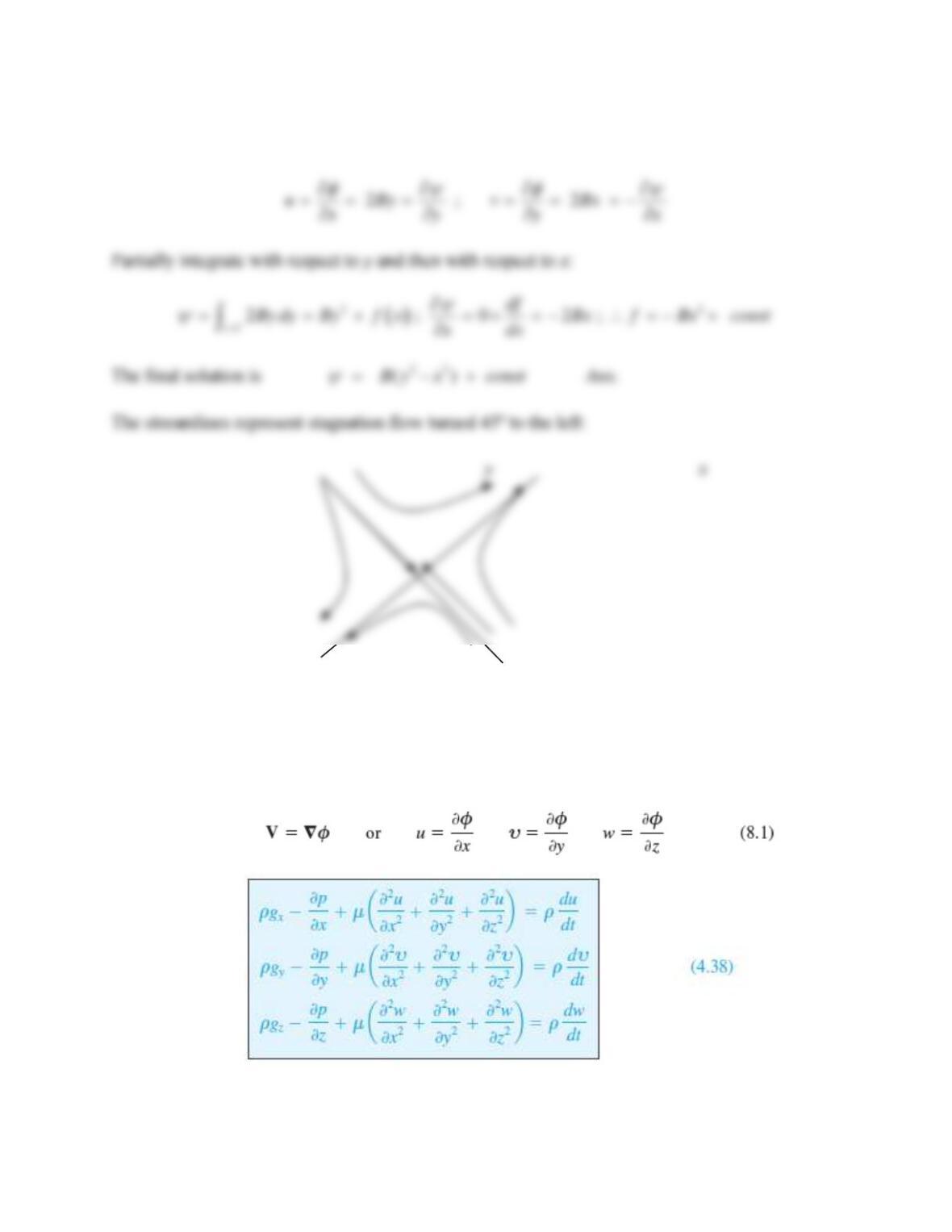
First find the velocities and relate them to the stream function:
Problem 8.7
Consider a flow with constant density and viscosity. If the flow possesses a velocity potential as
defined by Eq. (8.1), show that it exactly satisfies the full Navier-Stokes equation (4.38). If this
is so, why for inviscid theory do we back away from the full Navier-Stokes equations?
Solution 8.7
If V =
, the full Navier-Stokes equation is satisfied identically:
Problem 8.8
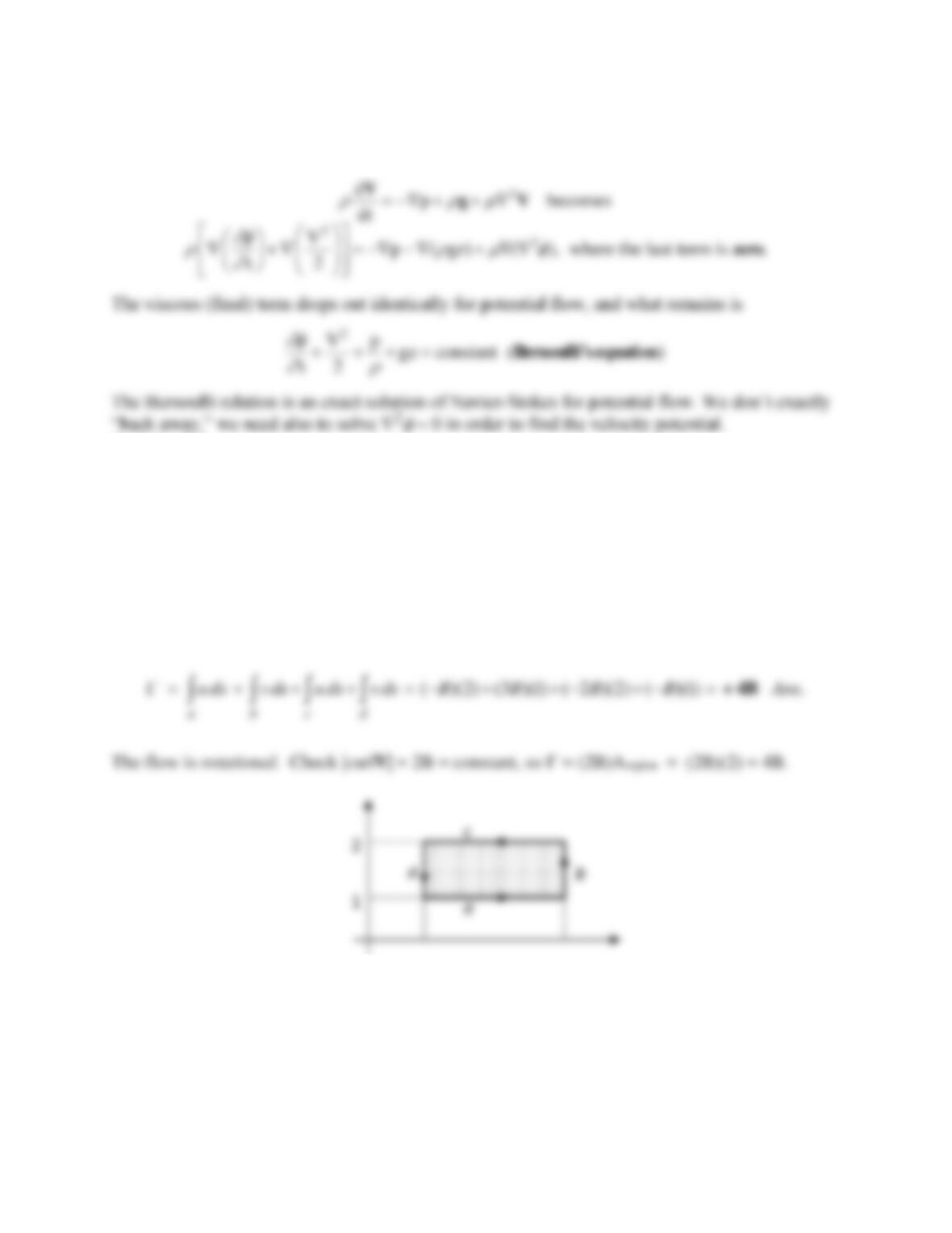
For the velocity distribution u = – B y, v = + B x, w = 0, evaluate the circulation about the
rectangular closed curve defined by (x, y) = (1,1), (3,1), (3,2), and (1,2). Interpret your result,
especially vis-à-vis the velocity potential.
Solution 8.8
Given that = V·ds around the curve, divide the rectangle into (a, b, c, d) pieces as shown
below.
Problem 8.9
Consider the two-dimensional flow u = –Ax, v = +Ay, where A is a constant. Evaluate the
circulation around the rectangular closed curve defined by (x, y) = (1, 1), (4, 1), (4, 3), and
(1, 3). Interpret your result especially vis-a-vis the velocity potential.
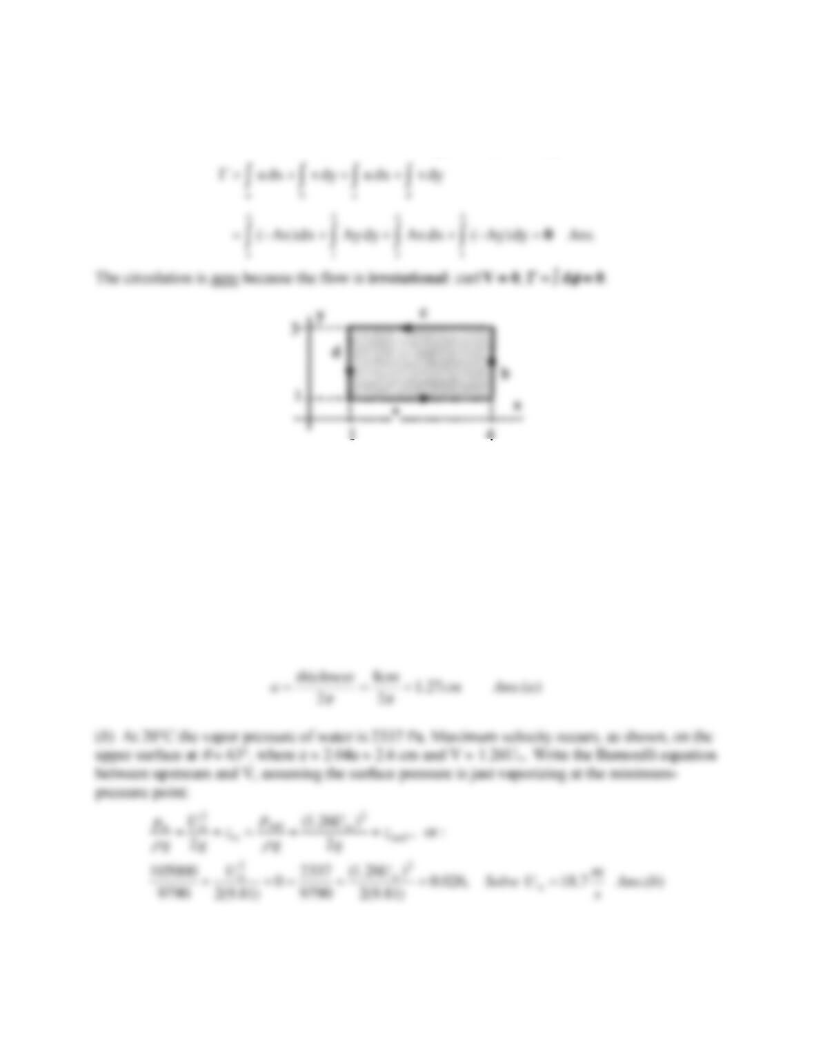
Solution 8.9
Given = V · ds around the curve, divide the rectangle into (a, b, c, d) pieces as shown below:
Problem 8.10
A two-dimensional Rankine half-body, 8 cm thick, is placed in a water tunnel at 20C. The water
pressure far up-stream along the body centerline is 105 kPa. (a) What is the nose radius of the
half-body? (b) At what tunnel flow velocity will cavitation bubbles begin to form on the surface
of the body?
Solution 8.10
(a) The nose radius is the distance a in Fig. 8.6, the Rankine half-body:
Problem 8.11
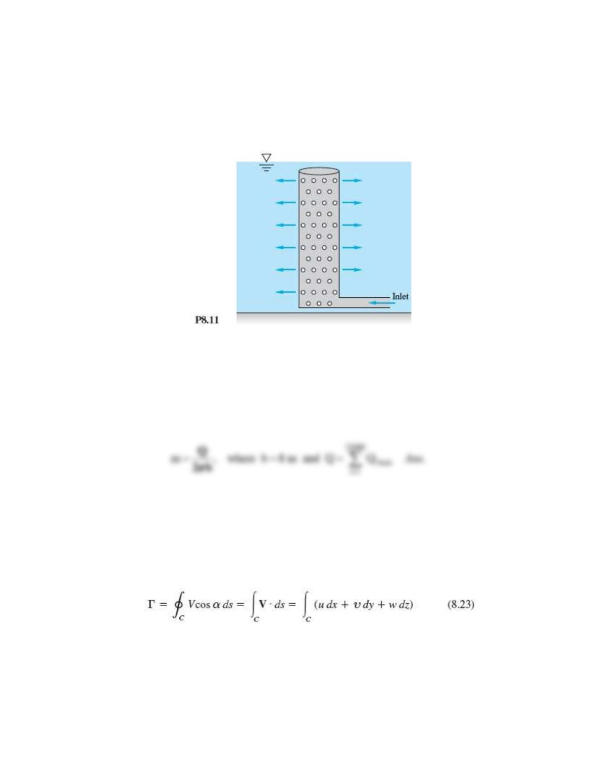
A power-plant discharges cooling water through the manifold in Fig. P8.11, which is 55 cm in
diameter and 8 m high and is perforated with 25,000 holes 1 cm in diameter. Does this manifold
simulate a line source? If so, what is the equivalent source strength m?
Solution 8.11
With that many small holes, equally distributed and presumably with equal flow rates, the
manifold does indeed simulate a line source of strength
Problem 8.12
Consider the flow due to a vortex of strength K at the origin. Evaluate the circulation from
Eq. (8.23) about the clockwise path from (a, 0) to (2a, 0) to (2a, 3
/2) to (a, 3
/2) and back to
(a, 0). Interpret the result.
Solution 8.12
Break the path up into (1, 2, 3, 4) as shown. Then
Problem 8.13
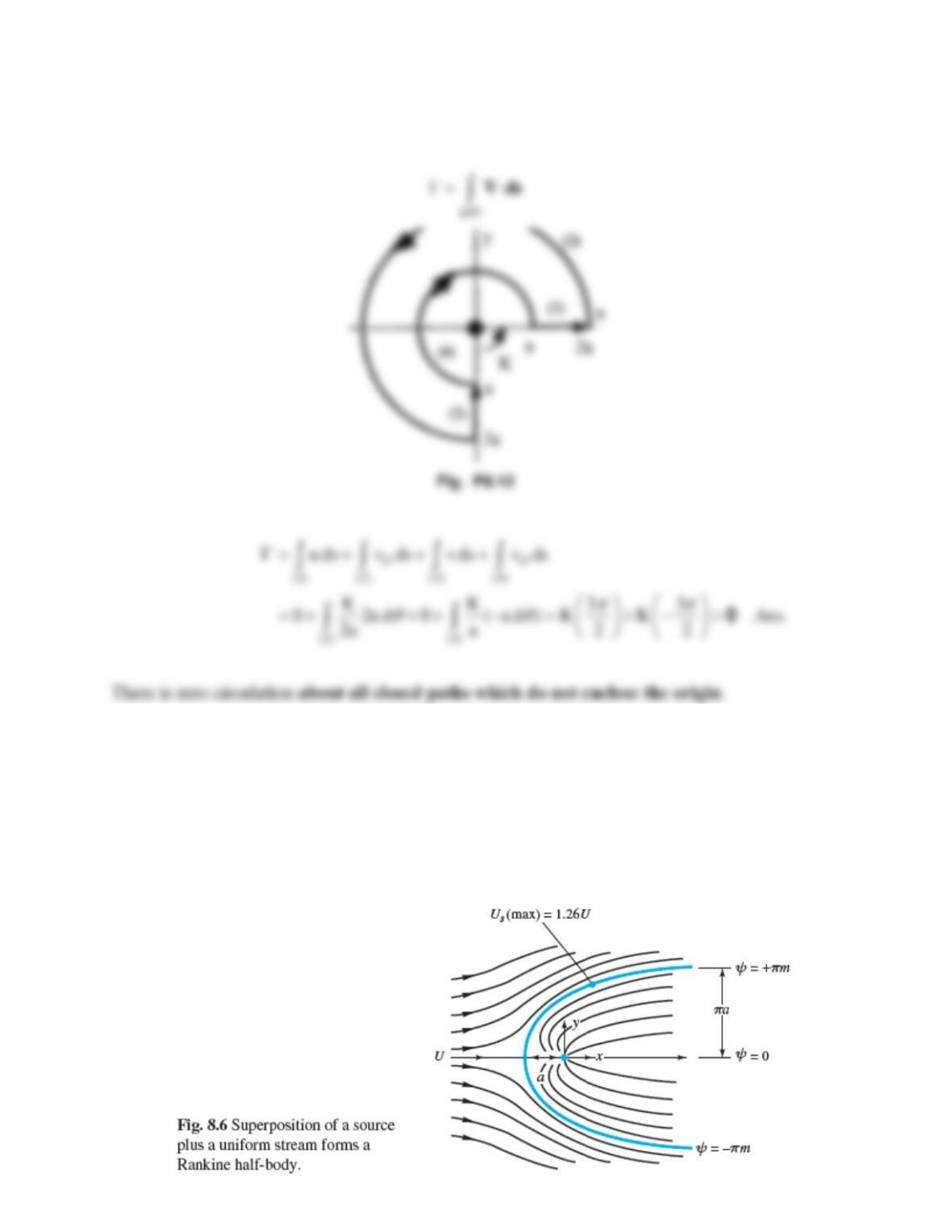
Starting at the stagnation point in Fig. 8.6, the fluid acceleration along the half-body surface
rises to a maximum and eventually drops off to zero far downstream. (a) Does this maximum
occur at the point in Fig. 8.6 where Umax = 1.26U? (b) If not, does the maximum acceleration
occur before or after that point? Explain.
Solution 8.13
Since the flow is steady, the fluid acceleration along the half-body surface is convective,
dU/dt = U(dU/ds), where s is along the surface. (a) At the point of maximum velocity in
Problem 8.14
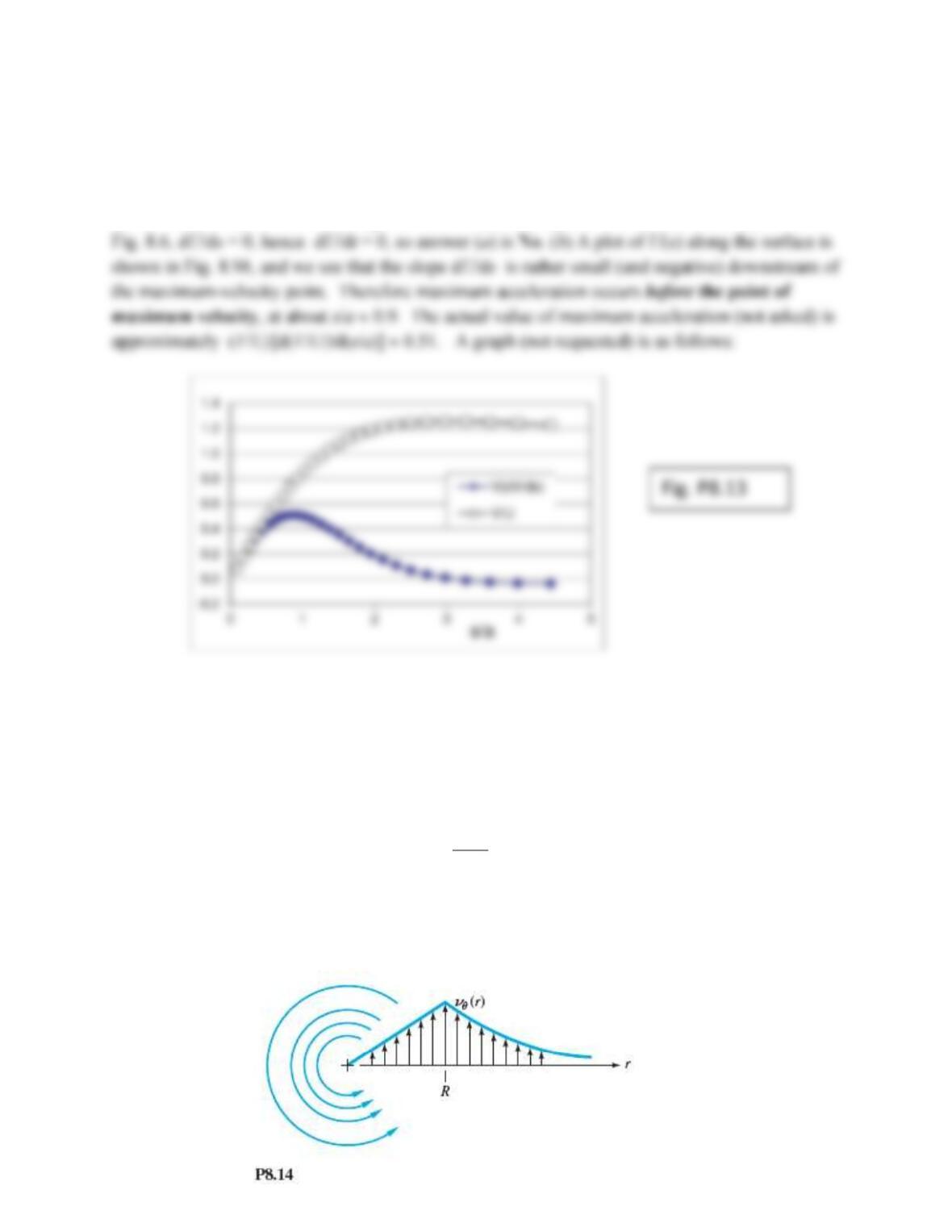
A tornado may be modeled as the circulating flow shown in Fig. P8.14, with
r =
z = 0 and
(r)
such that
2
r r R
RrR
r
=
Determine whether this flow pattern is irrotational in either the inner or outer region. Using the
r-momentum equation (D.5) of App. D, determine the pressure distribution p(r) in the tornado,
assuming p = p as r → Find the location and magnitude of the lowest pressure.
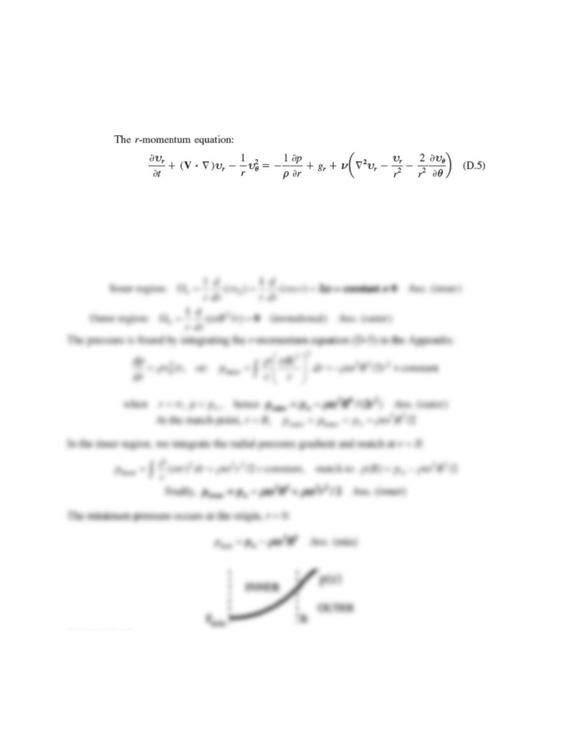
Solution 8.14
The inner region is solid-body rotation, the outer region is irrotational:
Problem 8.15
Hurricane Sandy, which hit the New Jersey coast on Oct. 29, 2012, was extremely broad, with
wind velocities of 40 mi/h at 400 miles from its center. Its maximum velocity was 90 mi/h.
Using the model of Fig. P8.14, at 20ºC with a pressure of 100 kPa far from the center, estimate
(a) the radius R of maximum velocity, in mi; and (b) the pressure at r = R.
Solution 8.15
The air density is p/RT = (100,000)/[287(293)] = 1.19 kg/m3. Convert 90 mi/h to 40.23 m/s and
40 mi/h to 17.9 m/s. The outer flow is irrotational, hence Bernoulli holds:
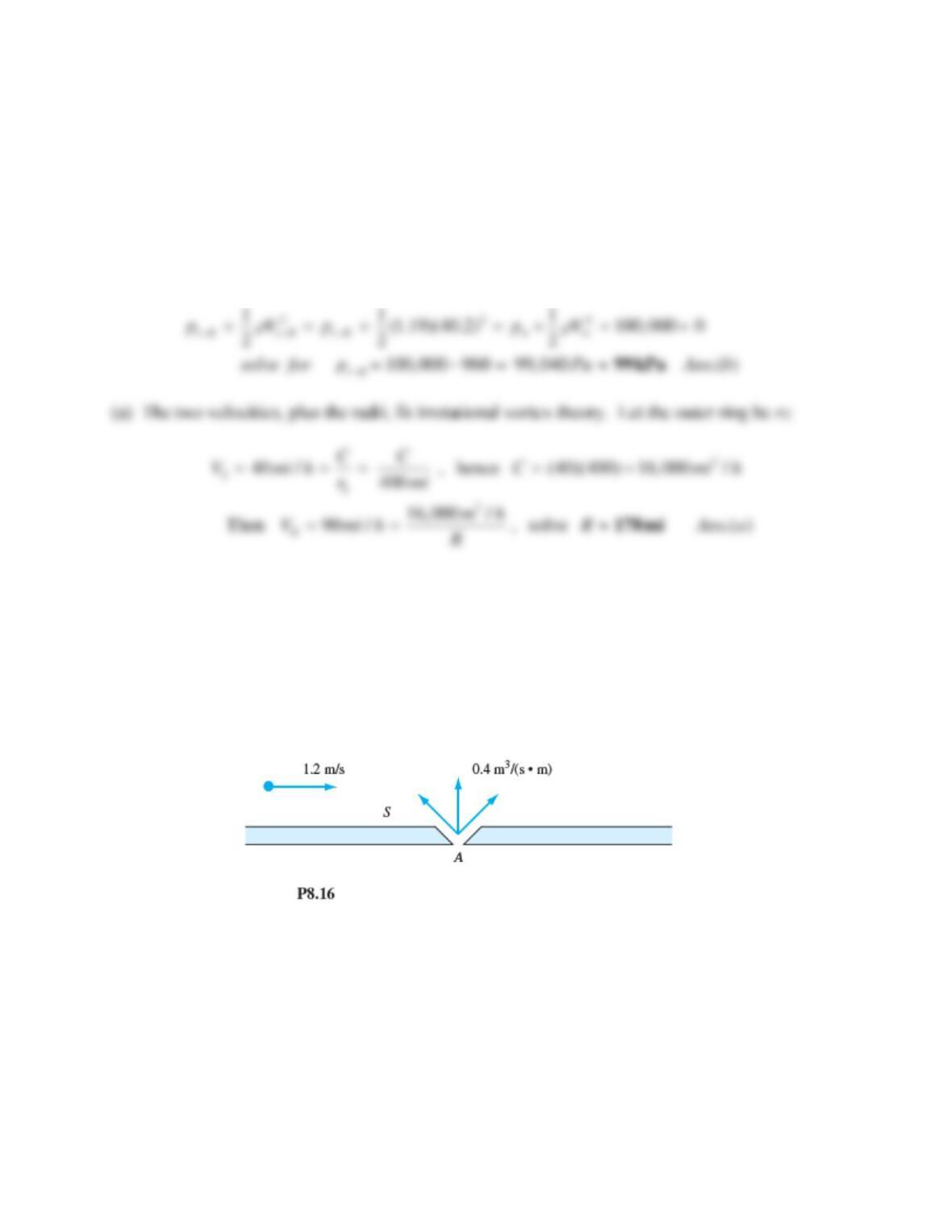
Problem 8.16
Air flows at 1.2 m/s along a flat surface when it encounters a jet of air issuing from the
horizontal wall at point A, as in Fig. P8.16. The jet volume flow is 0.4 m3/s per unit depth into
the paper. If the jet is approximated as an inviscid line source, (a) locate the stagnation point S on
the wall. (b) How far vertically will the jet flow extend into the stream?
Solution 8.16