Problem 7.C1
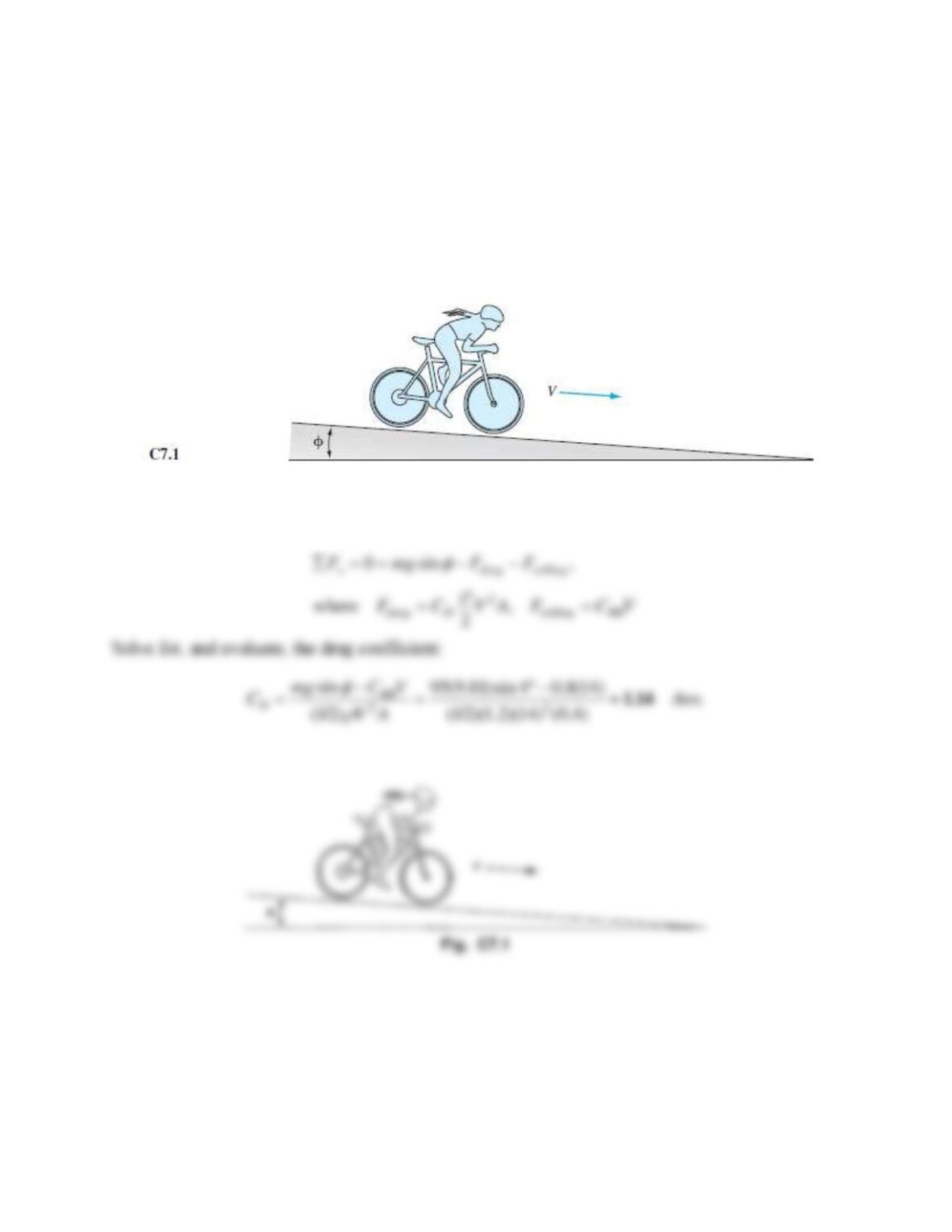
Jane wants to estimate the drag coefficient of herself on her bicycle. She measures the projected
frontal area to be 0.40 m2 and the rolling resistance to be 0.80 N · s/m. The mass of the bike is
15 kg, while the mass of Jane is 80 kg. Jane coasts down a long hill that has a constant 4° slope.
(See Fig. C7.1.) She reaches a terminal (steady state) speed of 14 m/s down the hill. Estimate the
aerodynamic drag coefficient CD of the rider and bicycle combination.
Solution 7.C1
For air take
1.2 kg/m3. Let x be down the hill. Then a force balance is
Problem 7.C2
Air at 20C and 1 atm flows at Vavg = 5 m/s between long, smooth parallel heat-exchanger plates
10 cm apart, as in Fig. C7.2. It is proposed to add a number of widely spaced 1-cm-long thin
interrupter plates to increase the heat transfer, as shown. Although the channel flow is turbulent,
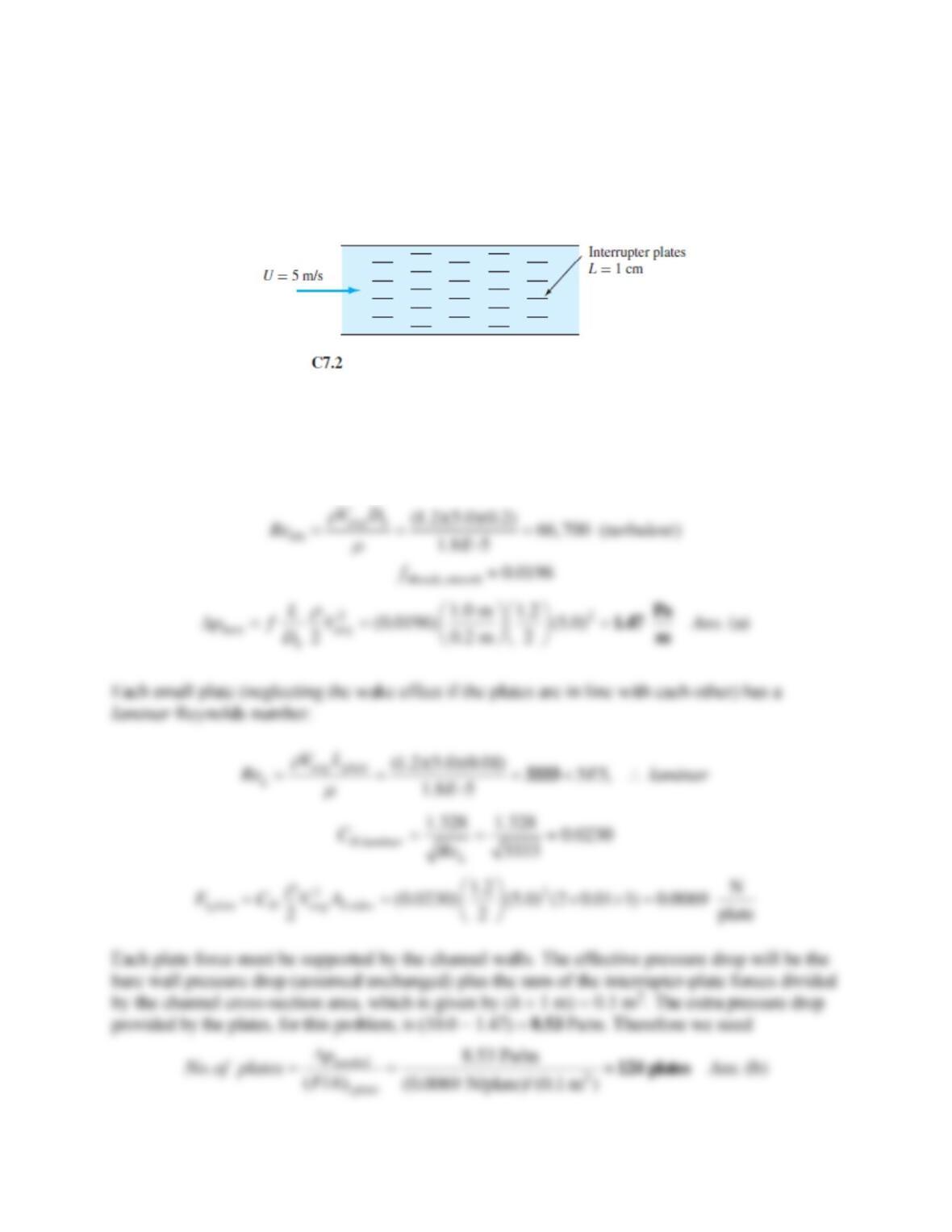
the boundary layer over the interrupter plates are essentially laminar. Assume all plates are 1 m
wide into the paper. Find (a) the pressure drop in Pa/m without the small plates present. Then
find (b) the number of small plates, per meter of channel length, that will cause the overall
pressure drop to be 10.0 Pa/m.
Solution 7.C2
For air, take
= 1.2 kg/m3 and
= 1.8E−5 kg/ms. (a) For wide plates, the hydraulic diameter is
Dh = 2h = 20 cm. The Reynolds number, friction factor, and pressure drop for the bare channel
(no small plates) is:
Problem 7.C3
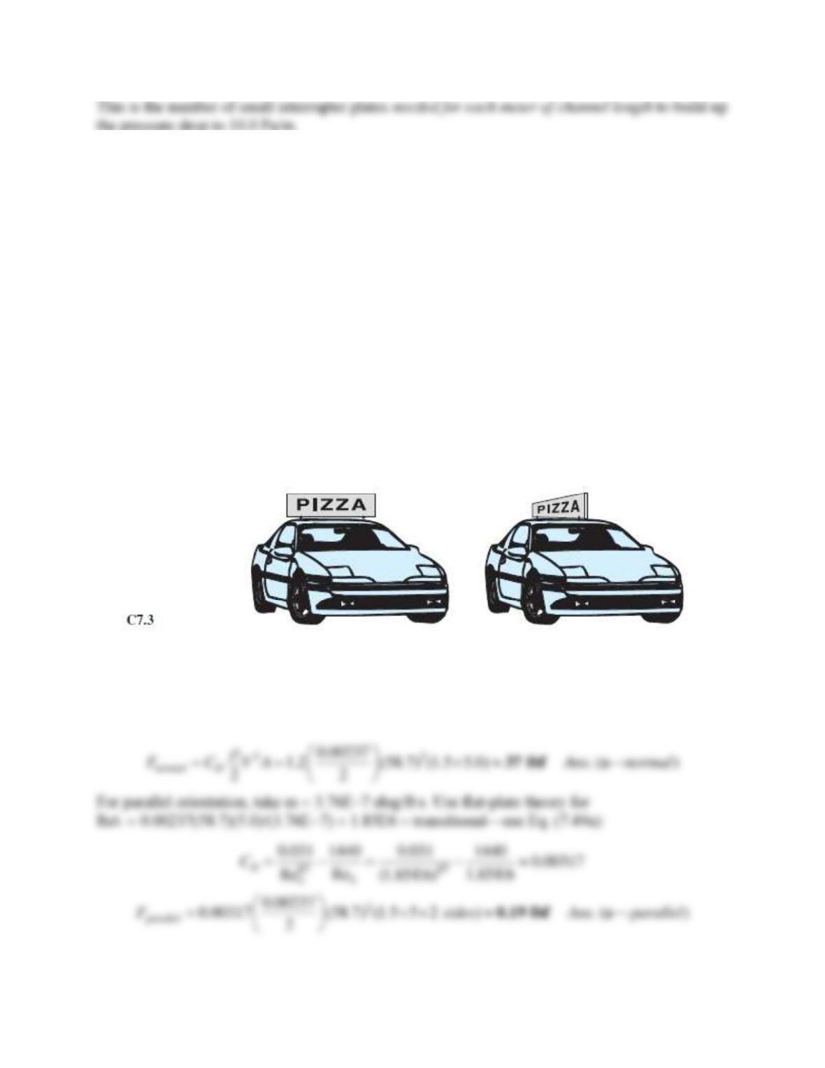
A new pizza store is planning to open. It will, of course, offer free delivery, and therefore need a
small delivery car with a large sign attached. The sign (a flat plate) is 1.5 ft high and 5 ft long.
The boss (having no feel for fluid mechanics) mounts the sign bluntly facing the wind. One of
his drivers is taking fluid mechanics and tells his boss he can save lots of money by mounting the
sign parallel to the wind. (See Fig. C7.3.) (a) Calculate the drag (in lbf) on the sign alone at
40 mi/h (58.7 ft/s) in both orientations. (b) Suppose the car without any sign has a drag
coefficient of 0.4 and a frontal area of 40 ft2. For V = 40 mi/h, calculate the total drag of the car–
sign combination for both orientations. (c) If the car has a rolling resistance of 40 lbf at 40 mi/h,
calculate the horsepower required by the engine to drive the car at 40 mi/h in both orientations.
(d) Finally, if the engine can deliver 10 hp for 1 h on a gallon of gasoline, calculate the fuel
efficiency in mi/gal for both orientations at 40 mi/h.
Solution 7.C3
For air take
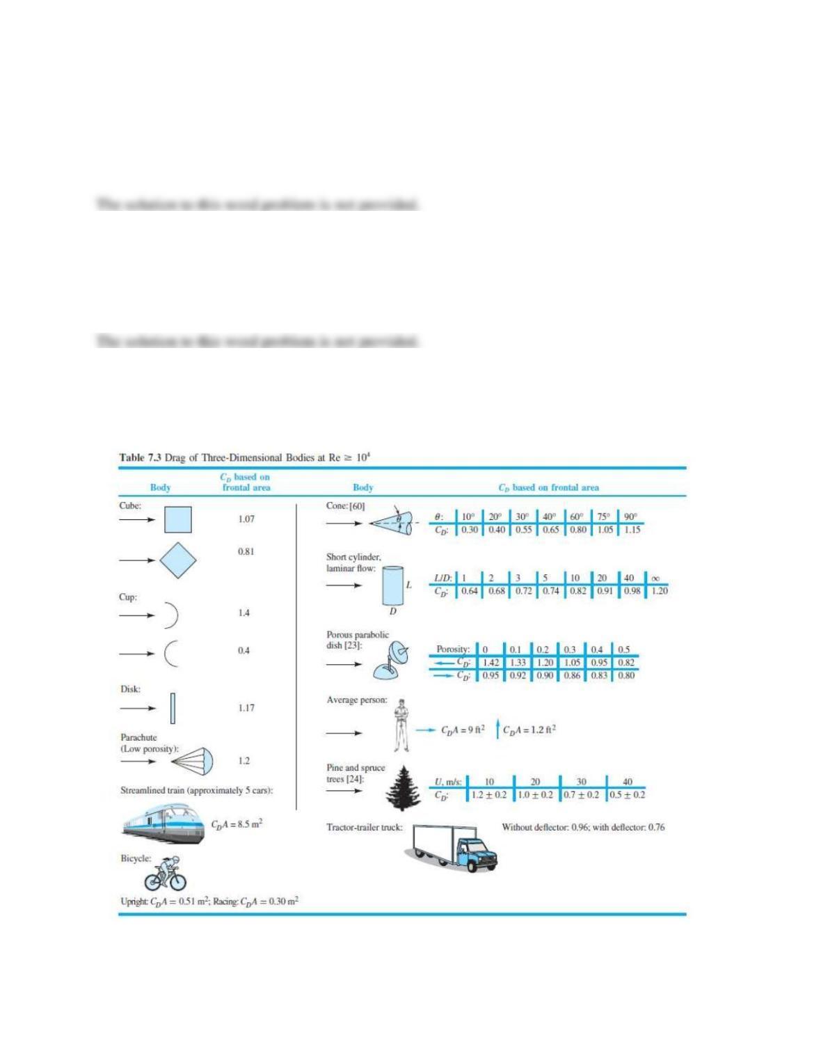
= 0.00237 slug/ft3. (a) Table 7.3, blunt plate, CD 1.2:
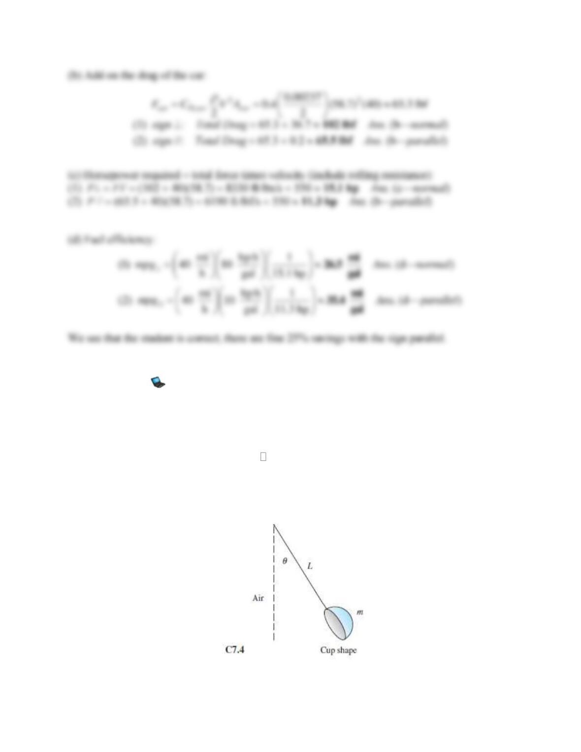
Problem 7.C4
Consider a pendulum with an unusual bob shape: a hemispherical cup of diameter D whose axis
is in the plane of oscillation, as in Fig. C7.4. Neglect the mass and drag of the rod L. (a) Set up
the differential equation for the oscillation
(t) and (b) nondimensionalize this equation.
(c) Determine the natural frequency for
1.
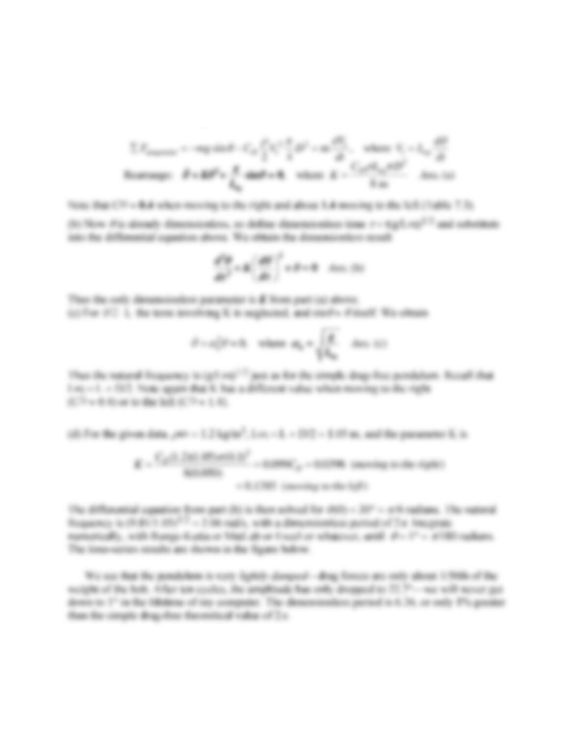
(d) For the special case L = 1 m, D = 10 cm,
m = 50 g, and air at 20C and 1 atm, and
(0) = 30, find (numerically) the time required for the
oscillation amplitude to drop to 1.
Solution 7.C4
(a) Let Leq = L + D/2 be the effective length of the pendulum. Sum forces in the direction of the
motion of the bob and rearrange into the basic 2nd-order equation:
Problem 7.C5
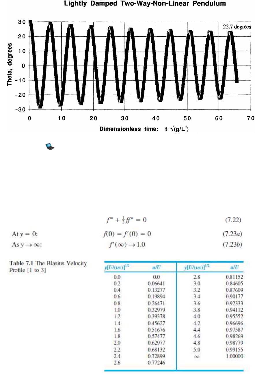
Program a method of numerical solution of the Blasius flatplate relation, Eq. (7.22), subject to
the conditions in Eqs. (7.23). You will find that you cannot get started without knowing the
initial second derivative f”(0), which lies between 0.2 and 0.5. Devise an iteration scheme that
starts at f”(0) ≈ 0.2 and converges to the correct value. Print out u/U = f ‘(η) and compare with
Table 7.1.
Solution 7.C5
Problem 7.W1
How do you recognize a boundary layer? Cite some physical properties and some measurements
that reveal appropriate characteristics.
Solution 7.W1
Problem 7.W2
In Chap. 6 the Reynolds number for transition to turbulence in pipe flow was about Retr ≈ 2300,
whereas in flatplate flow Retr ≈ 1 E6, nearly three orders of magnitude higher. What accounts for
the difference?
Solution 7.W2
Problem 7.W3
Without writing any equations, give a verbal description of boundary layer displacement
thickness.
Solution 7.W3
Problem 7.W4
Describe, in words only, the basic ideas behind the “boundary layer approximations.”
Solution 7.W4
Problem 7.W5
What is an adverse pressure gradient? Give three examples of flow regimes where such gradients
occur.
Solution 7.W5
Problem 7.W6
What is a favorable pressure gradient? Give three examples of flow regimes where such
gradients occur.
Solution 7.W6
Problem 7.W7
The drag of an airfoil (Fig. 7.12) increases considerably if you turn the sharp edge around
180 degrees to face the stream. Can you explain this?
Solution 7.W7
Problem 7.W8
In Table 7.3, the drag coefficient of a spruce tree decreases sharply with wind velocity. Can you
explain this?
Solution 7.W8
Problem 7.W9
Thrust is required to propel an airplane at a finite forward velocity. Does this imply an energy
loss to the system? Explain the concepts of thrust and drag in terms of the first law of
thermodynamics.
Solution 7.W9
The solution to this word problem is not provided.
Problem 7.W10
How does the concept of drafting, in automobile and bicycle racing, apply to the material studied
in this chapter?
Solution 7.W10
Problem 7.W11
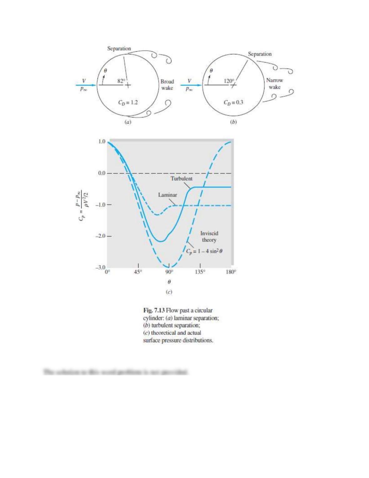
The circular cylinder of Fig. 7.13 is doubly symmetric and therefore should have no lift. Yet a
lift sensor would definitely reveal a finite root-mean-square value of lift. Can you explain this
behavior?
Solution 7.W11
Problem 7.W12
Explain in words why a thrown spinning ball moves in a curved trajectory. Give some physical
reasons why a side force is developed in addition to the drag.
Solution 7.W12
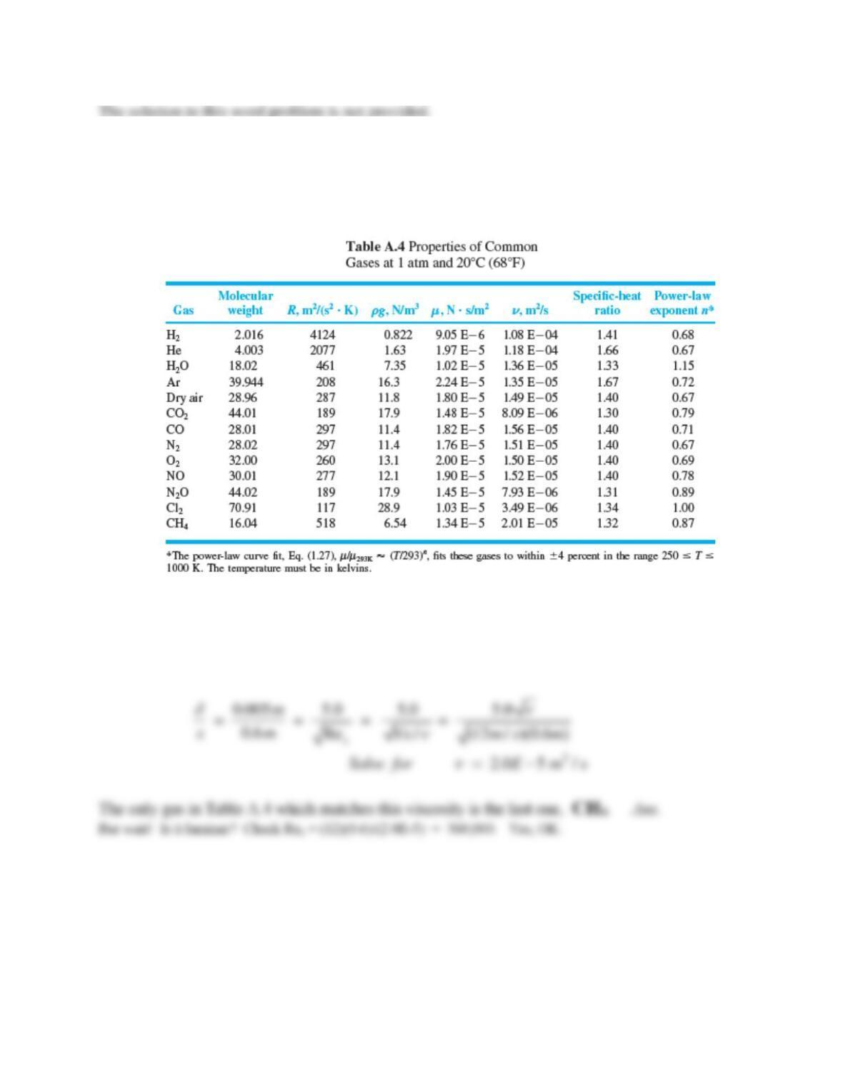
Problem 7.1
An ideal gas, at 20C and 1 atm, flows at 12 m/s past a thin flat plate. At a position 60 cm
downstream of the leading edge, the boundary layer thickness is 5 mm. Which of the 13 gases in
Table A.4 is this likely to be?
Solution 7.1
We are looking for the kinematic viscosity. For a gas at low velocity and a short distance, we
can guess laminar flow. Then we can begin by trying Eq. (7.1a):
Problem 7.2
A gas at 20ºC and 1 atm flows at 6 ft/s past a thin flat plate. At x = 3 ft, the boundary layer
thickness is 0.052 ft. Assuming laminar flow, which of the gases in Table A.4 is this likely to
be?
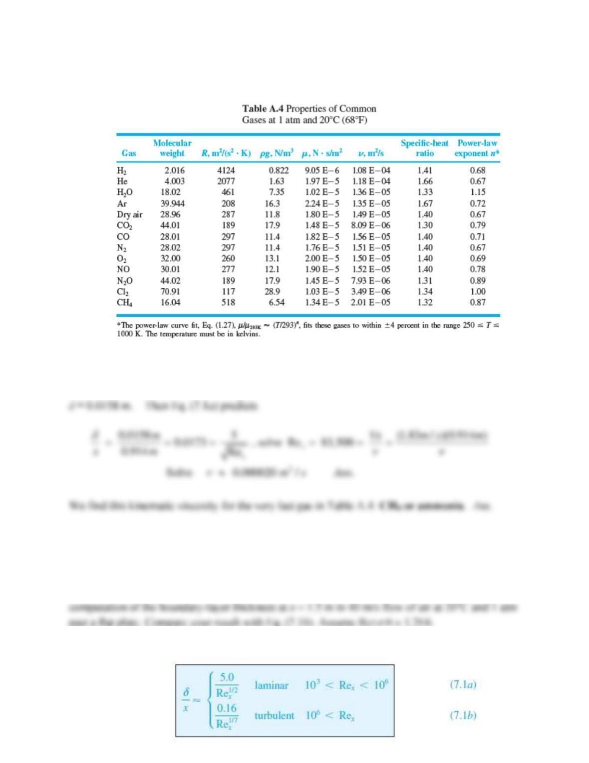
Solution 7.2
Since Table A.4 is metric, let’s change to SI units: x = 0.914 m, V =1.83 m/s, and
Problem 7.3
Equation (7.1b) assumes that the boundary layer on the plate is turbulent from the leading edge
onward. Devise a scheme for determining the boundary-layer thickness more accurately when
the flow is laminar up to a point Rex,crit and turbulent thereafter. Apply this scheme to
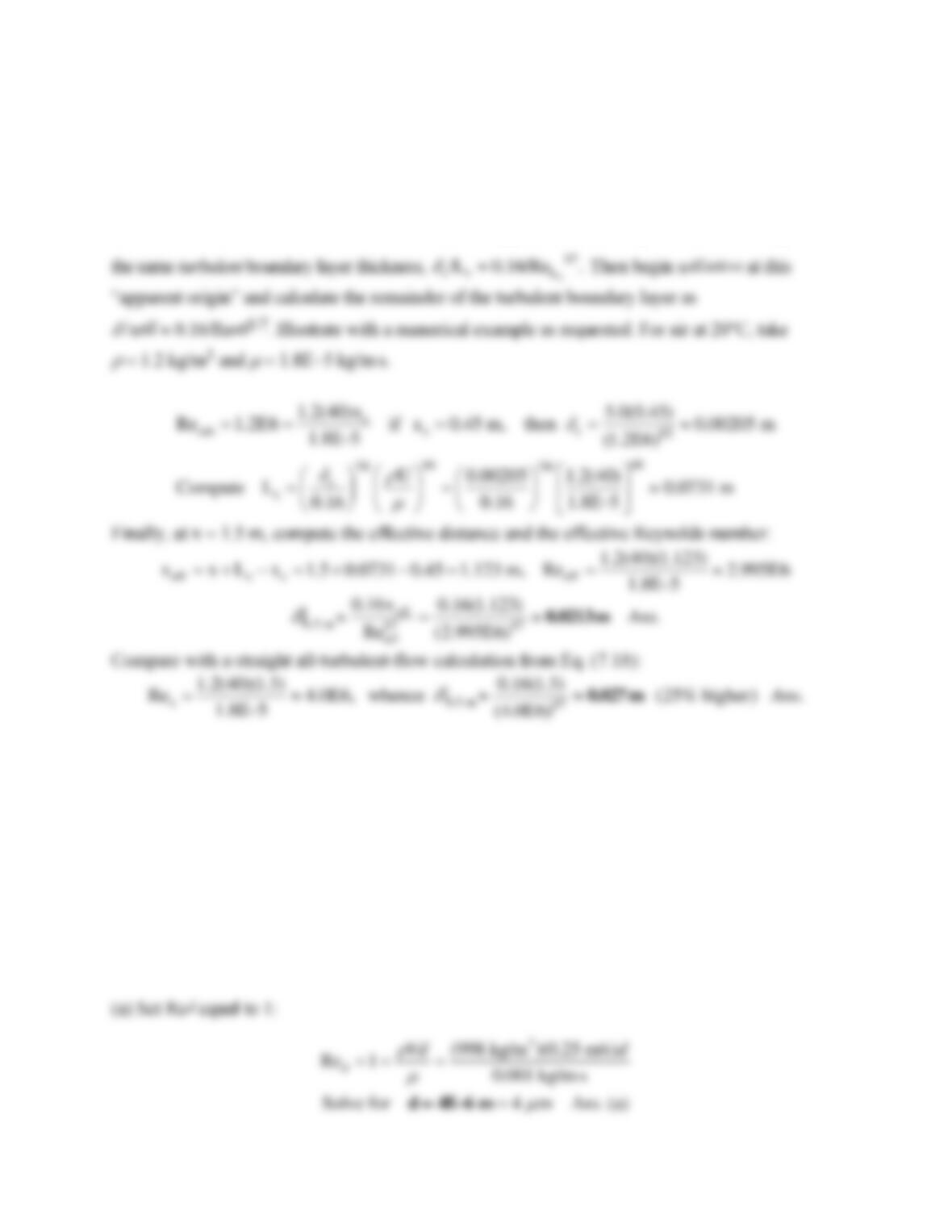
Solution 7.3
Given the transition point xcrit, Recrit, calculate the laminar boundary layer thickness
c at that point,
as shown above,
c/xc 5.0/Recrit1/2. Then find the “apparent” distance upstream, Lc, which gives
Problem 7.4
A smooth ceramic sphere (SG = 2.6) is immersed in a flow of water at 20C and 25 cm/s. What
is the sphere diameter if it is encountering (a) creeping motion, Red = 1; or (b) transition to
turbulence, Red = 250,000?
Solution 7.4
For water, take
= 998 kg/m3 and
= 0.001 kg/ms.
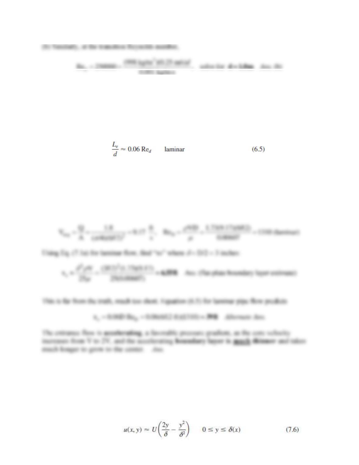
Problem 7.5
SAE 30 oil at 20C flows at 1.8 ft3/s from a reservoir into a 6–in–diameter pipe. Use flat–
plate theory to estimate the position x where the pipe–wall boundary layers meet in the
center. Compare with Eq. (6.5), and give some explanations for the discrepancy.
Solution 7.5
For SAE 30 oil at 20C, take
= 1.73 slug/ft3 and
= 0.00607 slug/fts. The average velocity
and pipe Reynolds number are:
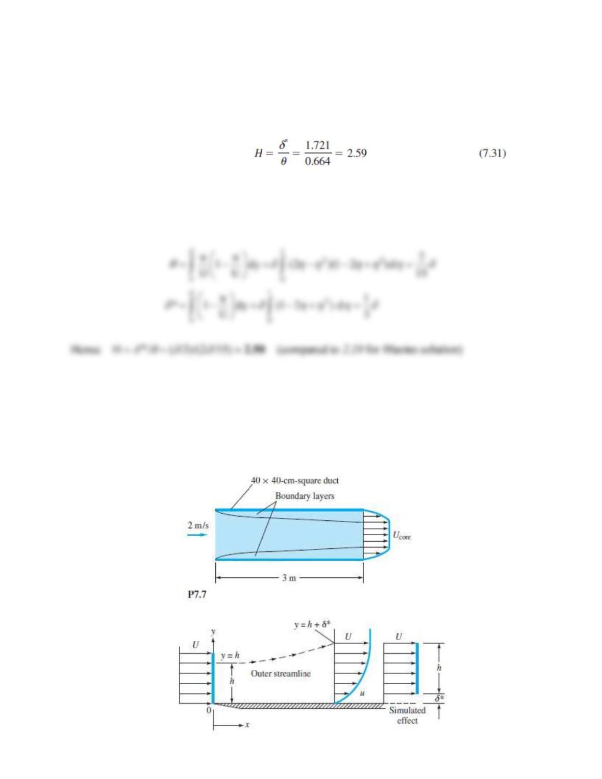
Problem 7.6
For the laminar parabolic boundary-layer profile of Eq. (7.6), compute the shape factor “H” and
compare with the exact Blasius theory result, Eq. (7.31).
Solution 7.6
Given the profile approximation u/U 2
−
2, where
= y/
, compute
Problem 7.7
Air at 20C and 1 atm enters a 40-cm-square duct as in Fig. P7.7. Using the “displacement
thickness” concept of Fig. 7.4, estimate (a) the mean velocity and (b) the mean pressure in the
core of the flow at the position x = 3 m. (c) What is the average gradient, in Pa/m, in this section?
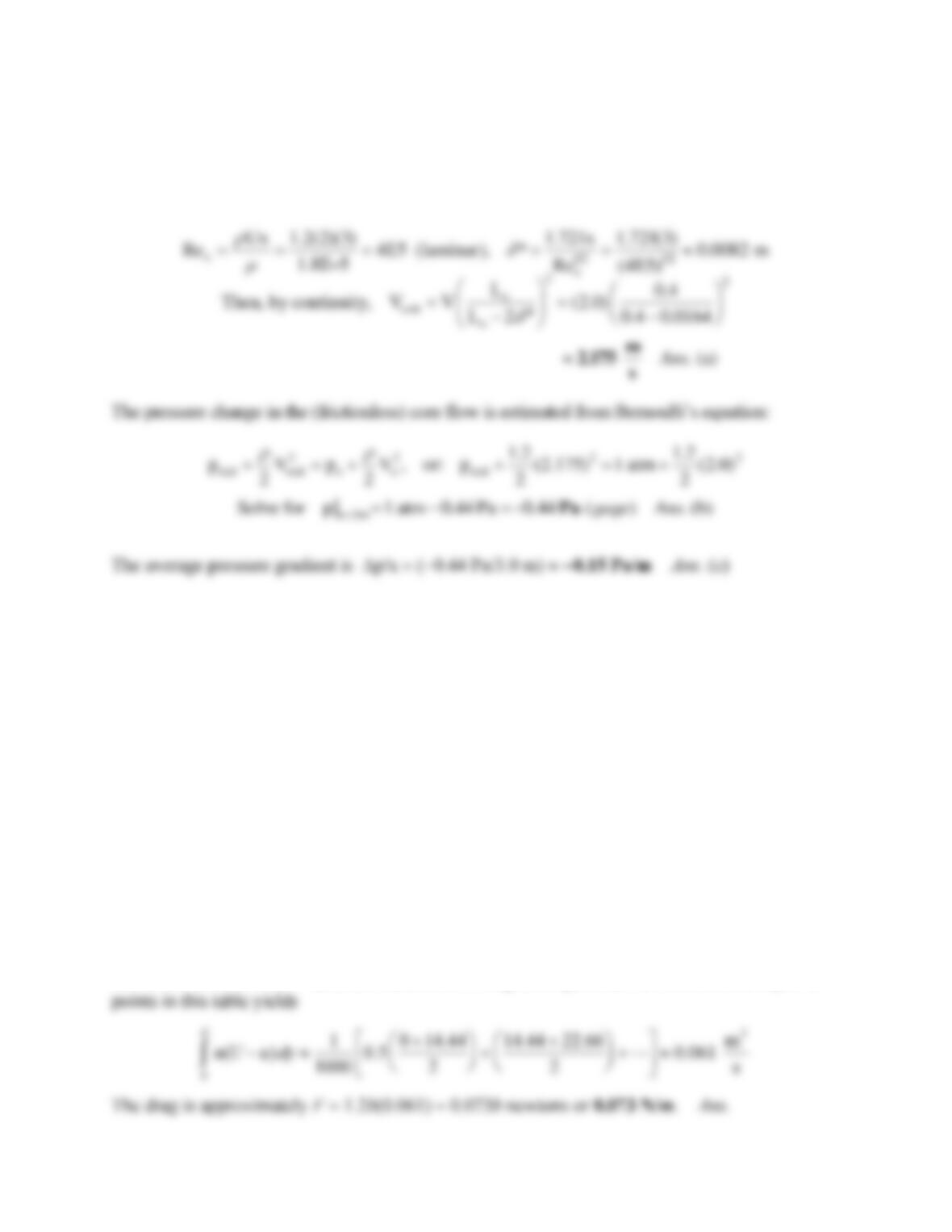
Solution 7.7
For air at 20C, take
= 1.2 kg/m3 and
= 1.8E−5 kg/ms. Using laminar boundary-layer
theory, compute the displacement thickness at x = 3 m:
Problem 7.8
Air,
=1.2 kg/m3 and
= 1.8E−5 kg/(ms), flows at 10 m/s past a flat plate. At the trailing edge
of the plate, the following velocity profile data are measured:
y, mm:
0
0.5
1.0
2.0
3.0
4.0
5.0
6.0
u, m/s:
0
1.75
3.47
6.58
8.70
9.68
10.0
10.0
If the upper surface has an area of 0.6 m2, estimate, using momentum concepts, the friction drag,
in N, on the upper surface.
Solution 7.8
Make a numerical estimate of drag from Eq. (7.2): F =
b
u(U
−
u)dy. We have added the
numerical values of u(U − u) to the data above. Using the trapezoidal rule between each pair of
Problem 7.9
Repeat the flat-plate momentum analysis of Sec. 7.2 by replacing Eq. (7.6) with the simple but
unrealistic linear velocity profile suggested by Schlichting [1]:
for 0
uy y
U
Compute momentum-integral estimates of cf,
/x,
*/x, and H.
Solution 7.9
Carry out the same integrations as Section 7.2. Results are less accurate:
Problem 7.10
Repeat Prob. P7.9, using a trigonometric profile approximation:
()
2
uy
sin
U
Does this profile satisfy the conditions of laminar flat plate flow?
Problem 7.9
Repeat the flat-plate momentum analysis of Sec. 7.2 by replacing Eq. (7.6) with the simple but
unrealistic linear velocity profile suggested by Schlichting [1]:
for 0
uy y
U
Compute momentum-integral estimates of cf,
/x,
*/x, and H.
Solution 7.10
Again carry out the integrations of Sec. 7.2:
0
4
(1 ) ( ) 0.1366
2
uu
dy
UU
−
= − =
Problem 7.11
Air at 20C and 1 atm flows at 2 m/s past a sharp flat plate. Assuming that Kármán’s parabolic-
profile analysis, Eqs. (7.6−7.10), is accurate, estimate (a) the local velocity u; and (b) the local
shear stress
at the position (x, y) = (50 cm, 5 mm).
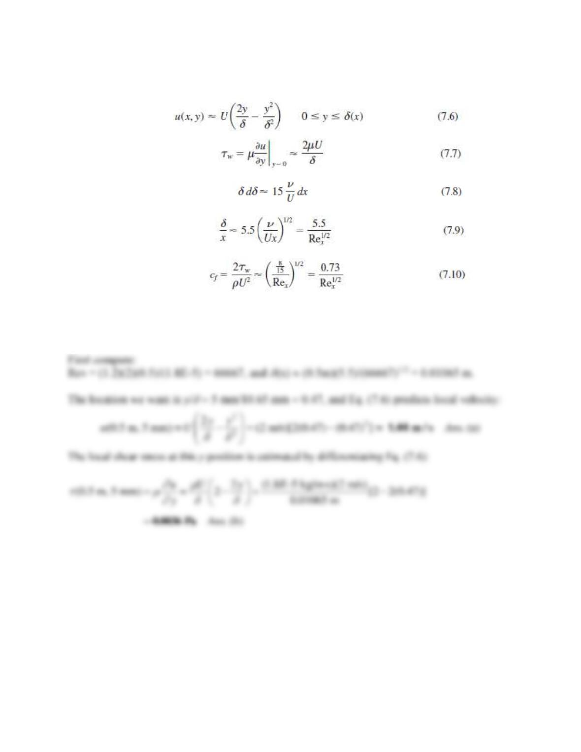
Solution 7.11
For air, take
= 1.2 kg/m3 and
= 1.8E−5 kg/ms.
Problem 7.12
The velocity profile shape u/U 1 − exp(−4.605y/
) is a smooth curve with u = 0 at y = 0 and
u = 0.99U at y =
and thus would seem to be a reasonable substitute for the parabolic flat-plate
profile of Eq. (7.3). Yet when this new profile is used in the integral analysis of Sec. 7.3, we get
the lousy result
1/2
/ 9.2/Rex
x
, which is 80 percent high. What is the reason for the inaccuracy?
[Hint: The answer lies in evaluating the laminar boundary-layer momentum equation (7.19b) at
the wall, y = 0.]
Solution 7.12
This profile satisfies no-slip at the wall and merges very smoothly with u → U at the outer edge,
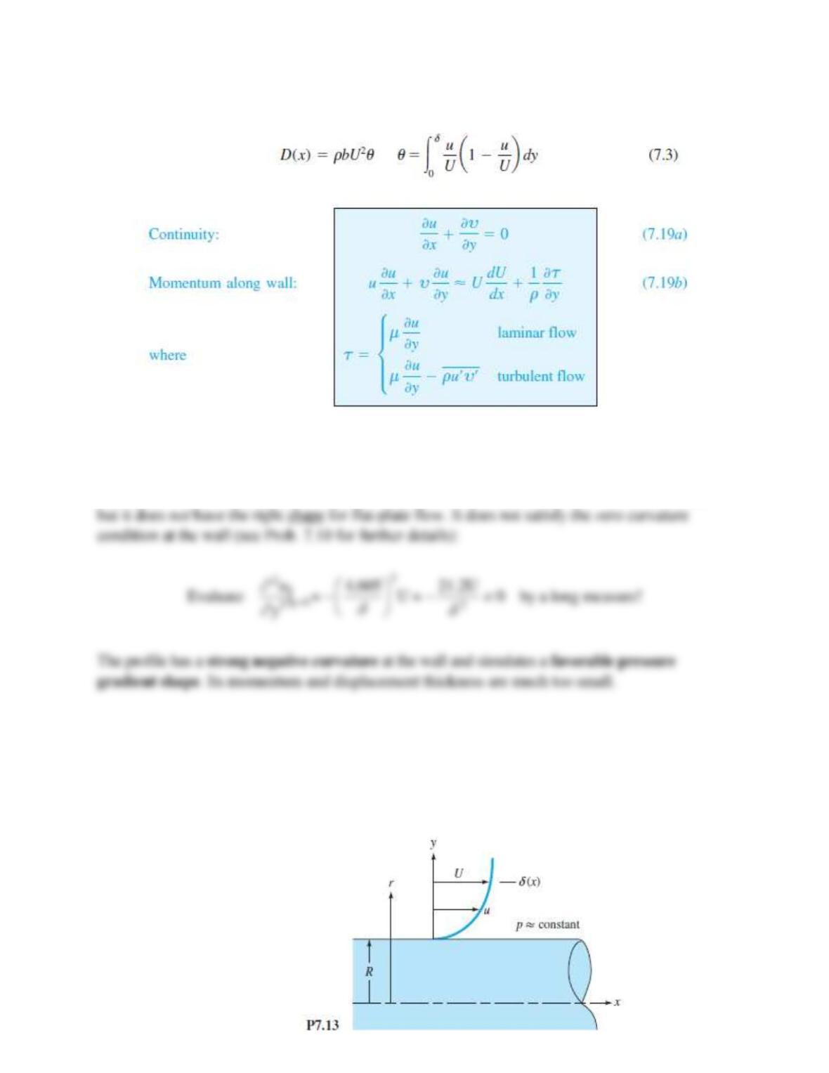
Problem 7.13
Derive modified forms of the laminar boundary-layer equations (7.19) for axisymmetric flow
along the outside of a circular cylinder of constant R, as in Fig. P7.13. Consider the two cases
(a)
R;
and (b)
R. What are the proper boundary conditions?