Atmospheric boundary layers are very thick but follow formulas very similar to those of flat-
plate theory. Consider wind blowing at 10 m/s at a height of 80 m above a smooth beach.
Estimate the wind shear stress, in Pa, on the beach if the air is standard sea-level conditions.
What will the wind velocity striking your nose be if (a) you are standing up and your nose is
170 cm off the ground; (b) you are lying on the beach and your nose is 17 cm off the ground?
Solution 7.38
For air at 20C, take
= 1.2 kg/m3 and
= 1.8E−5 kg/ms. Assume a smooth beach and use the
log-law velocity profile, Eq. (7.34), given u = 10 m/s at y = 80 m:
Problem 7.39
A hydrofoil 50 cm long and 4 m wide moves at 28 kn in seawater at 20C. Using flat-plate
theory with Retr = 5E5, estimate its drag, in N, for (a) a smooth wall and (b) a rough wall,
= 0.3 mm.
Solution 7.39
For seawater at 20C, take
= 1025 kg/m3 and
= 0.00107 kg/ms.
Problem 7.40
Hoerner [12, p. 3.25] states that the drag coefficient of a flag in winds, based on total wetted area
2bL, is approximated by CD ≈ 0.01 + 0.05L/b, where L is the flag length in the flow direction.
Test Reynolds numbers ReL were 1 E6 or greater. (a) Explain why, for L/b ≥ 1, these drag values
are much higher than for a flat plate. Assuming sea-level standard air at 50 mi/h, with area
bL = 4 m2, find (b) the proper flag dimensions for which the total drag is approximately 400 N.
Solution 7.40
(a) The drag is greater because the fluttering of the flag causes additional pressure drag on the
corrugated sections of the cloth. Ans. (a)
Problem 7.41
Repeat Prob. 7.20 with the sole change that the pitot probe is now 10 mm from the wall
(5 times higher). Show that the flow there cannot possibly be laminar, and use smooth–wall
turbulent–flow theory to estimate the position x of the probe, in m.
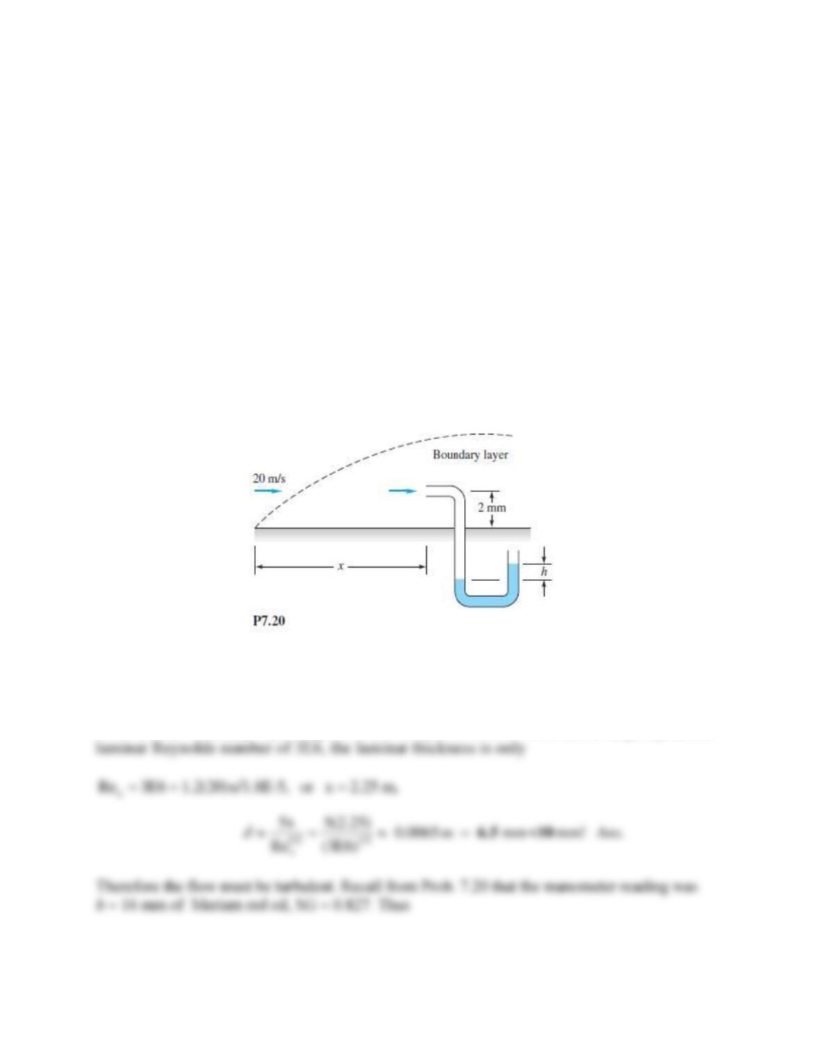
Problem 7.20
Air at 20C and 1 atm flows at 20 m/s past the flat plate in Fig. P7.20. A Pitot stagnation tube,
placed 2 mm from the wall, develops a manometer head h = 16 mm of Meriam red oil, SG = 0.827.
Use this information to estimate the downstream position x of the Pitot tube. Assume laminar
flow.
Solution 7.41
For air at 20C, take
= 1.2 kg/m3 and
= 1.8E−5 kg/ms. For U = 20 m/s, it is not possible
for a laminar boundary–layer to grow to a thickness of 10 mm. Even at the largest possible
Problem 7.42
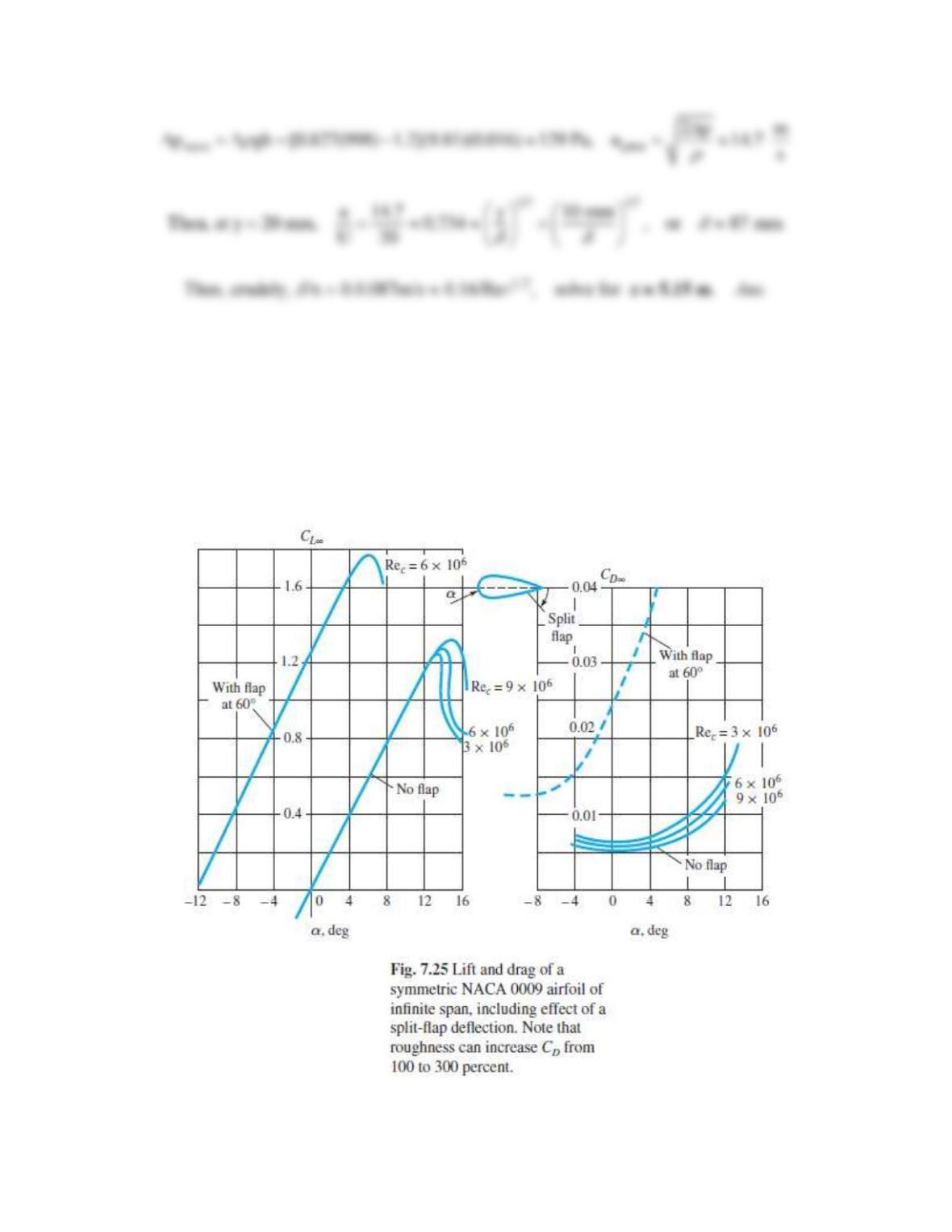
A light aircraft flies at 30 m/s in air at 20C and 1 atm. Its wing is an NACA 0009 airfoil, with a
chord length of 150 cm and a very wide span (neglect aspect ratio effects). Estimate the drag of
this wing, per unit span length, (a) by flat plate theory; and (b) using the data from Fig. 7.25 for
= 0.
Solution 7.42
For air at 20C and 1 atm,
= 1.2 kg/m3 and
= 1.8E-5 kg/m-s. First find the Reynolds
number, based on chord length, to see where we are:
36
(1.2 / )(30 / )(1.5 )
Re 3 10 turbulent
1.8E 5 /
c
Uc kg m m s m
kg m s
= = =
−−
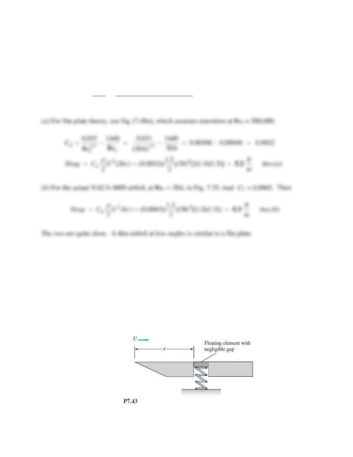
Problem 7.43
In the flow of air at 20C and 1 atm past a flat plate in Fig. P7.43, the wall shear is to be
determined at position x by a floating element (a small area connected to a strain-gage force
measurement). At x = 2 m, the element indicates a shear stress of 2.1 Pa. Assuming turbulent
flow from the leading edge, estimate (a) the stream velocity U, (b) the boundary layer thickness
at the element, and (c) the boundary-layer velocity u, in m/s, at 5 mm above the element.
Solution 7.43
For air at 20C, take
= 1.2 kg/m3 and
= 1.8E−5 kg/ms. The shear stress is
Problem 7.44
Extensive measurements of wall shear stress and local velocity for turbulent airflow on the flat
surface of the University of Rhode Island wind tunnel have led to the following proposed
correlation:
1.77
2
20.0207
w
yuy
Thus, if y and u(y) are known at a point in a flat-plate boundary layer, the wall shear may be
computed directly. If the answer to part (c) of Prob. 7.43 is u 26.3 m/s, determine the shear
stress and compare with Prob. P7.43. Discuss.
Problem 7.43
In the flow of air at 20C and 1 atm past a flat plate in Fig. P7.43, the wall shear is to be
determined at position x by a floating element (a small area connected to a strain-gage force
measurement). At x = 2 m, the element indicates a shear stress of 2.1 Pa. Assuming turbulent
flow from the leading edge, estimate (a) the stream velocity U, (b) the boundary layer thickness
at the element, and (c) the boundary-layer velocity u, in m/s, at 5 mm above the element.
Solution 7.44
For air at 20C, take
= 1.2 kg/m3 and
= 1.8E−5 kg/ms. The shear stress is given as 2.1 Pa,
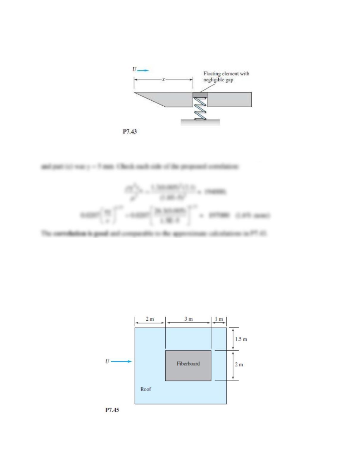
Problem 7.45
A thin sheet of fiberboard weighs 90 N and lies on a rooftop, as shown in Figure P7.45. Assume
ambient air at 20C and 1 atm. If the coefficient of solid friction between board and roof is
= 0.12,
what wind velocity will generate enough fluid friction to dislodge the board?
Solution 7.45
For air take
= 1.2 kg/m3 and
= 1.8E−5 kg/ms. Our first problem is to evaluate the drag when
Problem 7.46
A ship is 150 m long and has a wetted area of 5000 m2. If it is encrusted with barnacles, the ship
requires 7000 hp to overcome friction drag when moving in seawater at 15 kn and 20C. What is
the average roughness of the barnacles? How fast would the ship move with the same power if
the surface were smooth? Neglect wave drag.
Solution 7.46
For seawater at 20C, take
= 1025 kg/m3 and
= 0.00107 kg/ms. Convert
Problem 7.47
Local boundary layer effects, such as shear stress and heat transfer, are best correlated with local
variables, rather using distance x from the leading edge. The momentum thickness
is often
used as a length scale. Use the analysis of turbulent flat-plate flow to write local wall shear
stress
w in terms of dimensionless
and compare with the formula recommended by
Schlichting [1]: Cf 0.033 Re
–0.268.
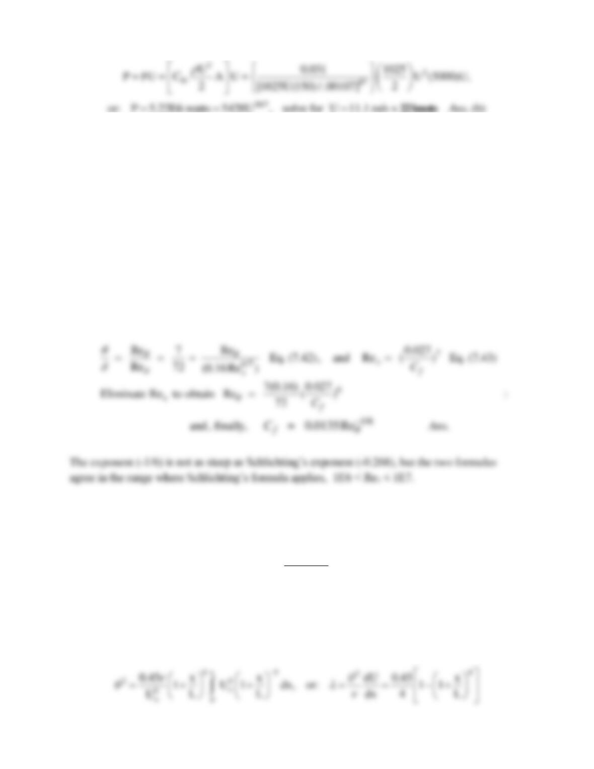
Solution 7.47
Our turbulent flat-plate theory, Eqs. (7.40) to (7.43), has expressions for Cf and
in terms of
Rex. Eliminate Rex to solve for Cf in terms of Re
Problem 7.48
In 1957 H. Görtler proposed the adverse gradient test cases
o
(1 / )n
U
UxL
=+
and computed separation for laminar flow at n = 1 to be xsep/L = 0.159. Compare with Thwaites’
method, assuming
o = 0.
Solution 7.48
Introduce this stream velocity (n = 1) into Eq. (7.54), with
o = 0, and integrate:
sep
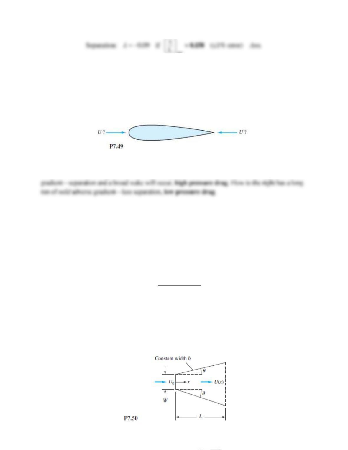
Problem 7.49
Based strictly on your understanding of flat-plate theory plus adverse and favorable pressure
gradients, explain the direction (left or right) for which airflow past the slender airfoil shape in
Fig. P7.49 will have lower total (friction 1 pressure) drag.
Solution 7.49
Flow to the left has a long run of mild favorable gradient and then a short run of strong adverse
Problem 7.50
Consider the flat-walled diffuser in Fig. P7.50, which is similar to that of Fig. 6.26a with
constant width b. If x is measured from the inlet and the wall boundary layers are thin, show that
the core velocity U(x) in the diffuser is given approximately by
o
1 (2 tan )/
U
UxW
=+
where W is the inlet height. Use this velocity distribution with Thwaite’s method to compute the
wall angle
for which laminar separation will occur in the exit plane when diffuser length
L = 2W. Note that the result is independent of the Reynolds number.
Solution 7.50
We can approximate U(x) by the one-dimensional continuity relation:
Problem 7.51
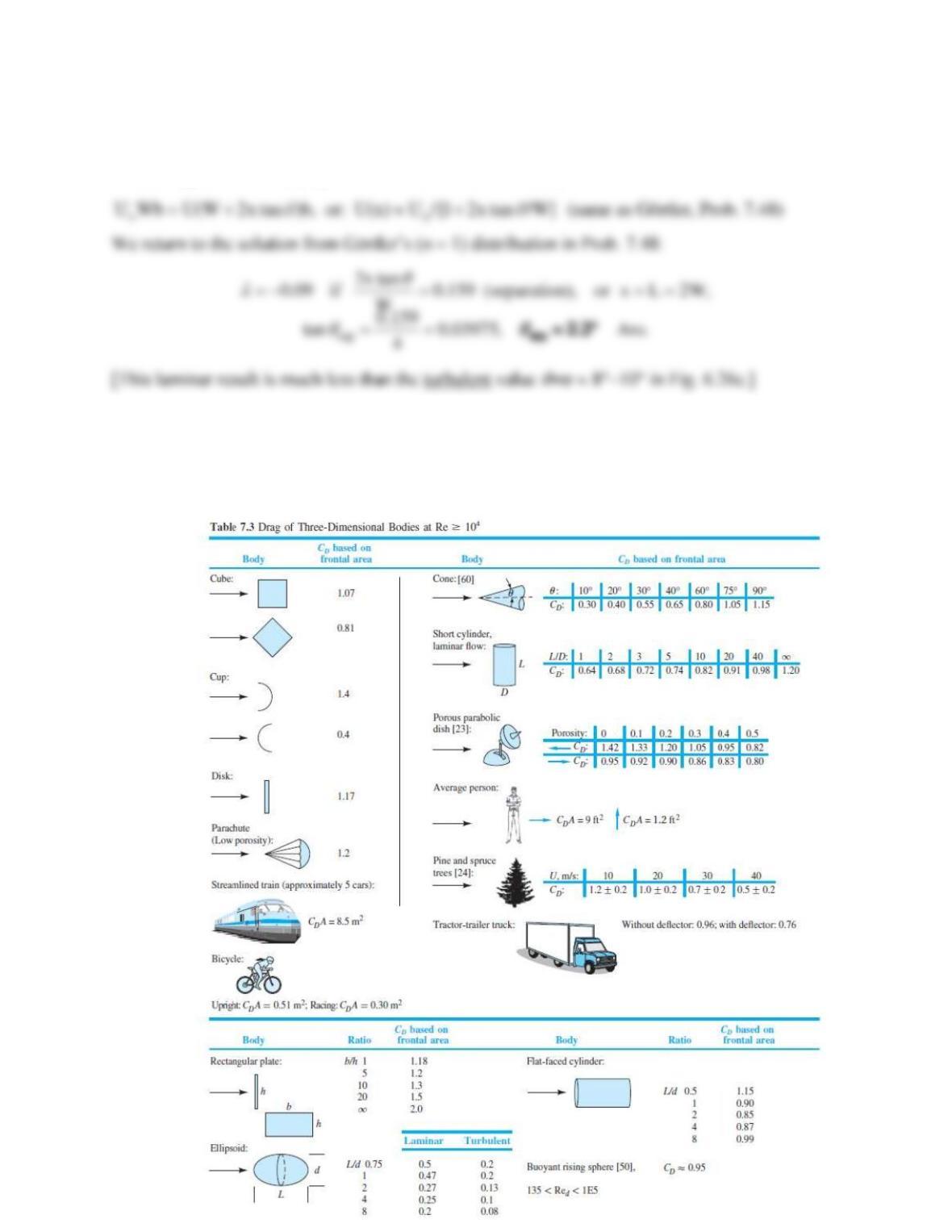
A 2-cm-diameter solid metal sphere falls steadily at about 1 m/s in 20ºC fresh water. If we use
Table 7.3 for a drag estimate, is the sphere made of steel, aluminum, or copper?
Solution 7.51
Approximate specific gravities: Steel 7.8, Aluminum 2.7, copper 8.9. Check the Reynolds
number for water, ρ = 998 kg/m3 and μ = 0.0010 kg/m∙s:
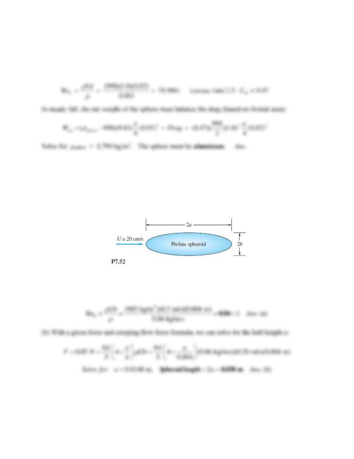
Problem 7.52
Clift et al. [46] give the formula F (6
/5)(4 + a/b)
Ub for the drag of a prolate spheroid in
creeping motion, as shown in Fig. P7.52. The half-thickness b is 4 mm. If the fluid is SAE 50W
oil at 20C, (a) check that Reb < 1; and (b) estimate the spheroid length if the drag is 0.02 N.
Solution 7.52
For SAE 50W oil, take
= 902 kg/m3 and
= 0.86 kg/ms. (a) The Reynolds number based on
half-thickness is:
Problem 7.53
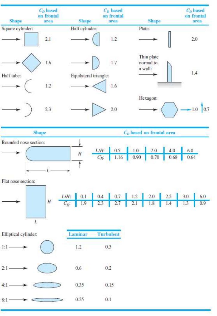
From Table 7.2, the drag coefficient of a wide plate normal to a stream is approximately 2.0. Let the
stream conditions be U and p. If the average pressure on the front of the plate is approximately
equal to the free-stream stagnation pressure, what is the average pressure on the rear?
Table 7.2 Drag of Two-Dimensional Bodies at Re ≥ 104
Solution 7.53
If the drag coefficient is 2.0, then our approximation is
Problem 7.54
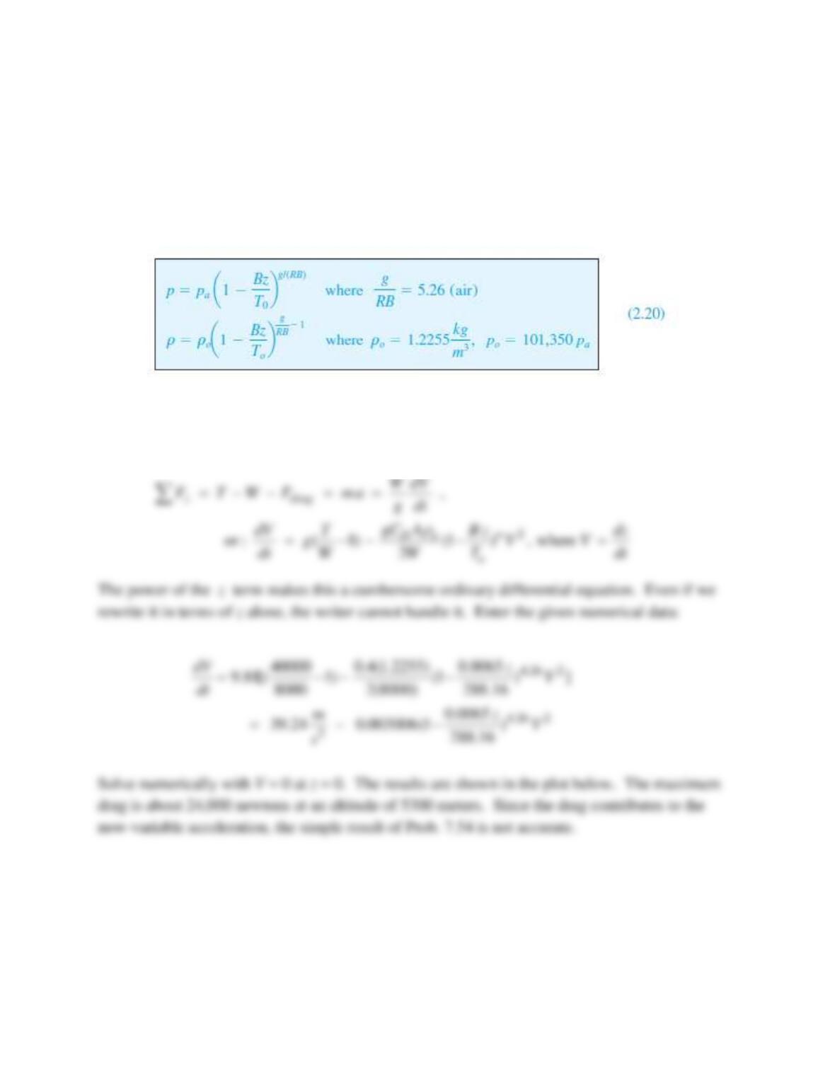
If a missile takes off vertically from sea level and leaves the atmosphere, it has zero drag when it
starts and zero drag when it finishes. It follows that the drag must be a maximum somewhere in
between. To simplify the analysis, assume a constant drag coefficient, CD, and a constant
vertical acceleration, a. Let the density variation be modeled by the troposphere relation,
Eq. (2.20). Find an expression for the altitude z* where the drag is a maximum. Comment on
your result.
Solution 7.54
For constant acceleration and CD, the drag follows simple formulas:
Problem 7.55
A ship tows a submerged cylinder, 1.5 m in diameter and 22 m long, at U = 5 m/s in fresh water
at 20C. Estimate the towing power in kW if the cylinder is (a) parallel, and (b) normal to the
tow direction.
Solution 7.55
For water at 20C, take
= 998 kg/m3 and
= 0.001 kg/ms.
L D,frontal
L 998(5)(22)
(a) Parallel, 15, Re 1.1E8, Table 7.3: estimate C 1.1
D 0.001
= =
22
998
F 1.1 (5) (1.5) 24000 N, Power FU (a)
24 Ans.
= =
120 kW
D D,frontal
998(5)(1.5)
(b) Normal, Re 7.5E6, Fig. 7.16a: C 0.4
0.001
= =
2
998
F 0.4 (5) (1.5)(22) 165000 N, Power FU (b)
2Ans.
= =
800 kW
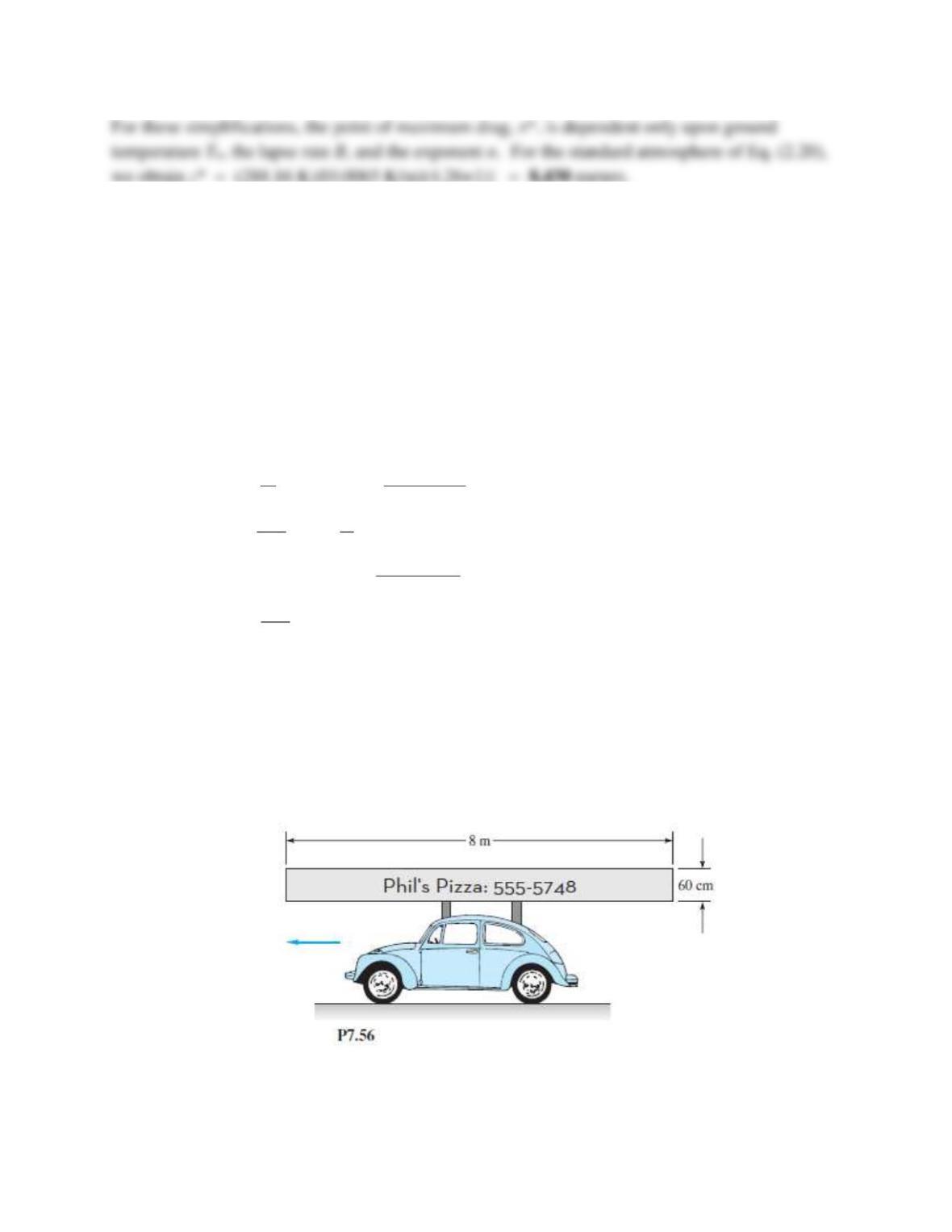
Problem 7.56
A delivery vehicle carries a long sign on top, as in Fig. P7.56. If the sign is very thin and the
vehicle moves at 65 mi/h, (a) estimate the force on the sign with no crosswind. (b) Discuss the
effect of a crosswind.
Solution 7.56
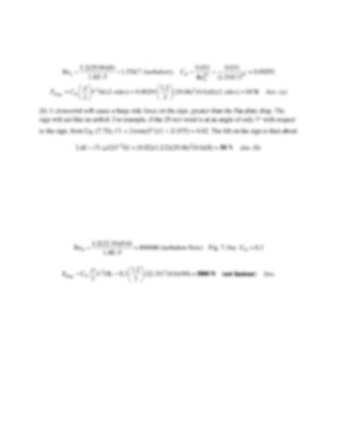
For air at 20C, take
= 1.2 kg/m3 and
= 1.8E−5 kg/ms. Convert 65 mi/h = 29.06 m/s. (a) If there
is no crosswind, we may estimate the drag force by flat-plate theory:
Problem 7.57
The main cross-cable between towers of a coastal suspension bridge is 60 cm in diameter and
90 m long. Estimate the total drag force on this cable in crosswinds of 50 mi/h. Are these
laminar-flow conditions?
Solution 7.57
For air at 20C, take
= 1.2 kg/m3 and
= 1.8E−5 kg/ms. Convert 50 mi/h = 22.35 m/s. Check
the Reynolds number of the cable:
Problem 7.58*
Modify Prob. P7.54 to be more realistic by accounting for missile drag during ascent. Assume
constant thrust T and missile weight W. Neglect the variation of g with altitude. Solve for the
altitude z* in the standard atmosphere where the drag is a maximum, for T = 40,000 N,
W = 8,000 N, and CDA = 0.4 m2. The writer does not believe an analytic solution is practical.
Problem 7.54
If a missile takes off vertically from sea level and leaves the atmosphere, it has zero drag when it
starts and zero drag when it finishes. It follows that the drag must be a maximum somewhere in
between. To simplify the analysis, assume a constant drag coefficient, CD, and a constant
vertical acceleration, a. Let the density variation be modeled by the troposphere relation,
Eq. (2.20). Find an expression for the altitude z* where the drag is a maximum. Comment on
your result.
Solution 7.58*
Summation of vertical forces gives the (variable) acceleration:
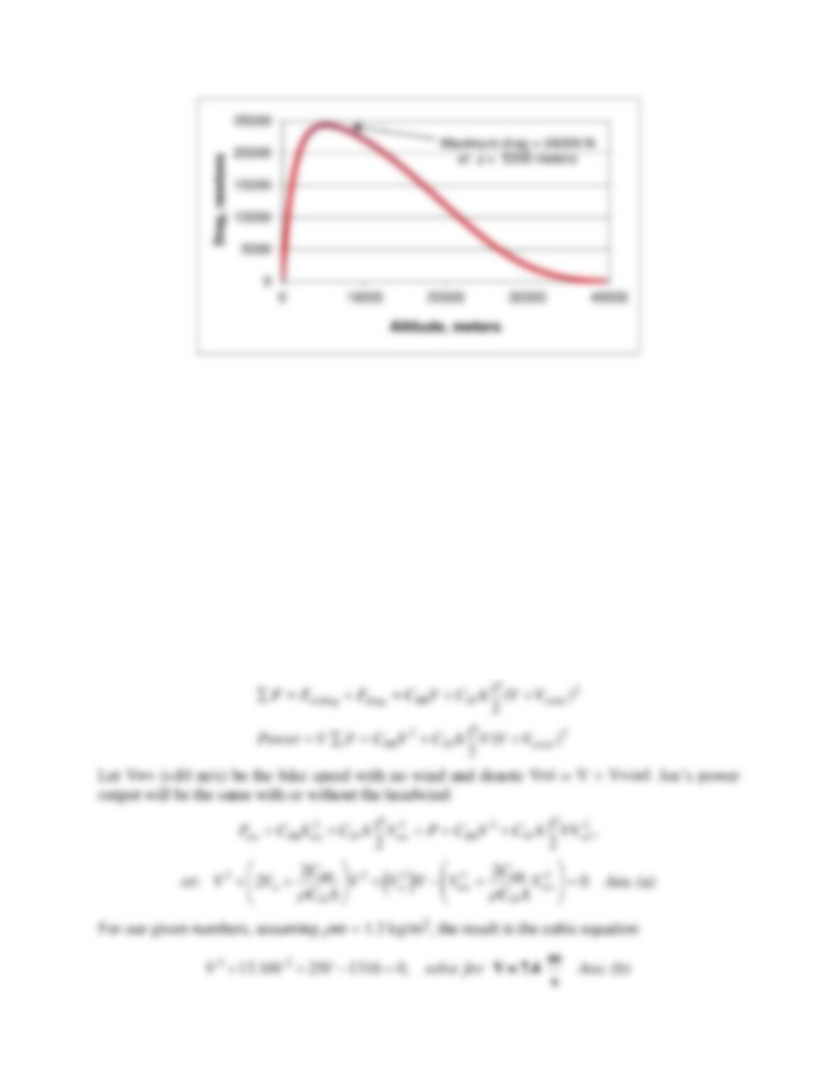
Problem 7.59*
Joe can pedal his bike at 10 m/s on a straight, level road with no wind. The rolling resistance of
his bike is 0.80 N/(m/s), that is 0.8 N per m/s of speed. The drag area CDA of Joe and his bike is
0.422 m2. Joe’s mass is 80 kg and that of the bike is 15 kg. He now encounters a head wind of
5.0 m/s. (a) Develop an equation for the speed at which Joe can pedal into the wind. (Hint: A
cubic equation for V will result.) (b) Solve for V: that is, how fast can Joe ride into the
headwind? (c) Why is the result not simply 10 − 5.0 = 5.0 m/s, as one might first suspect?
Solution 7.59*
Evaluate force and power with the drag based on relative velocity V + Vwind:
Problem 7.60
A fishnet consists of 1-mm–diameter strings overlapped and knotted to form 1- by 1-cm squares.
Estimate the drag of 1 m2 of such a net when towed normal to its plane at 3 m/s in 20C seawater.
What horsepower is required to tow 400 ft2 of this net?
Solution 7.60
For seawater at 20C, take
=1025 kg/m3 and
= 0.00107 kg/ms. Neglect the knots at the net’s
intersections. Estimate the drag of a single one-centimeter strand:
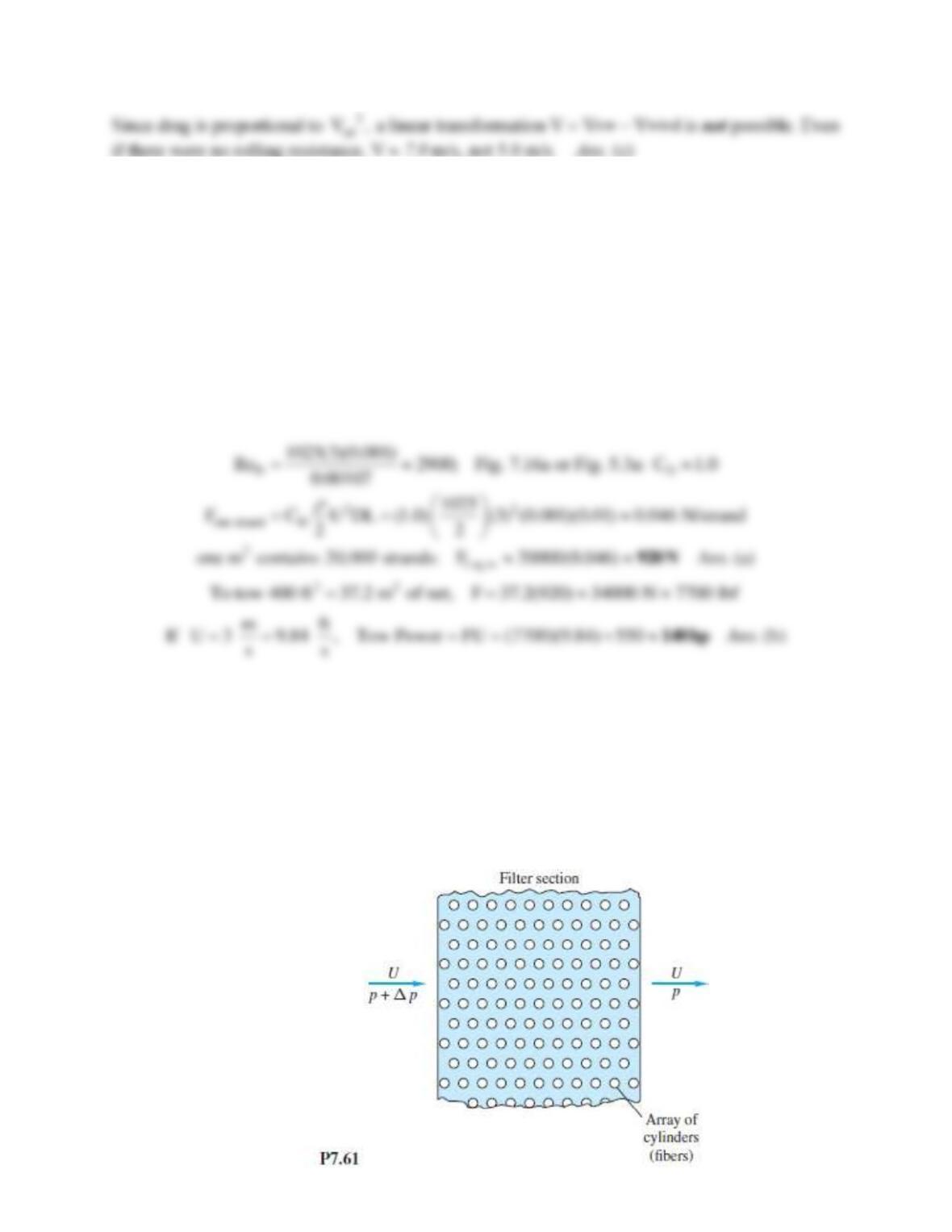
Problem 7.61
A filter may be idealized as an array of cylindrical fibers normal to the flow, as in Fig. P7.61.
Assuming that the fibers are uniformly distributed and have drag coefficients given by Fig 7.16a,
derive an approximate expression for the pressure drop p through a filter of thickness L.
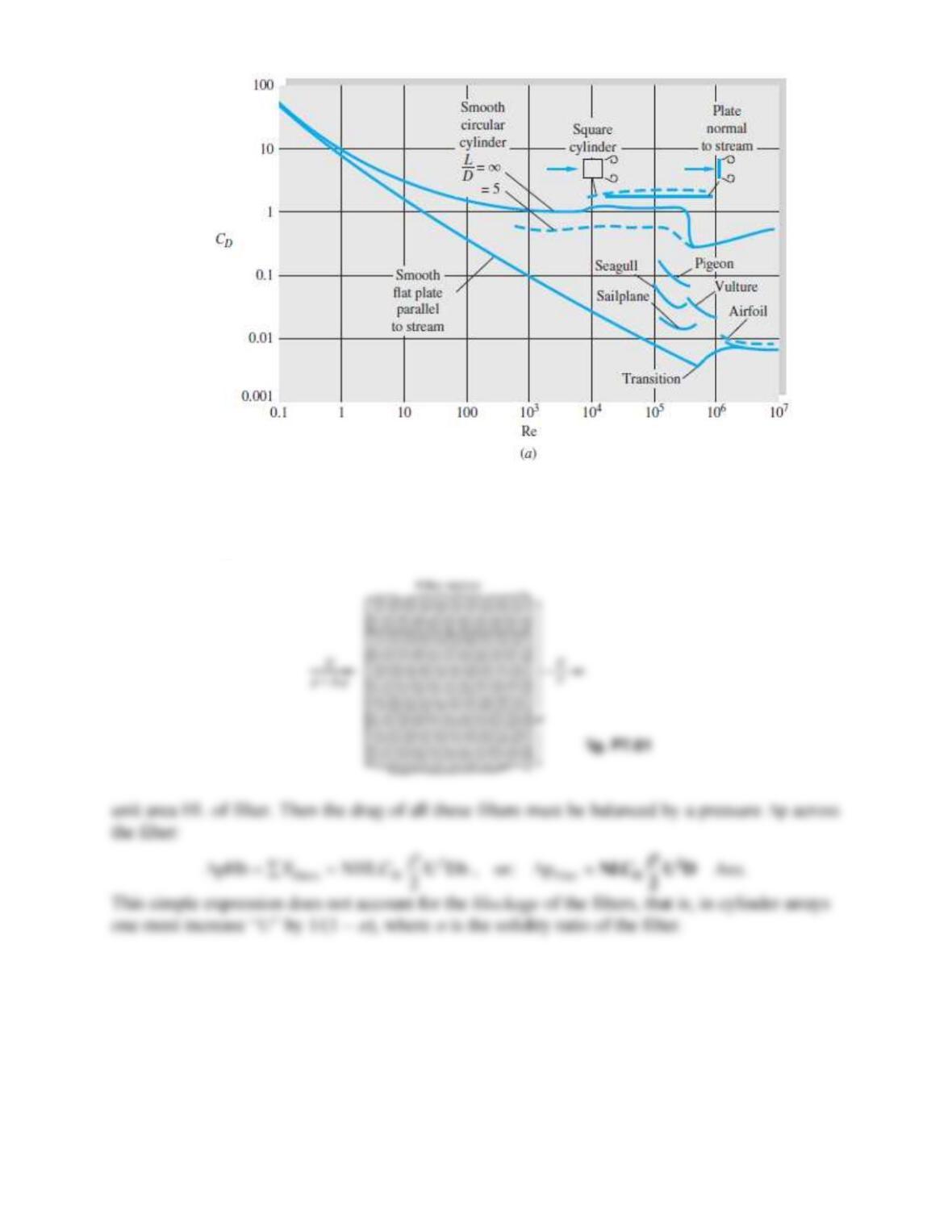
Solution 7.61
Consider a filter section of height H and width b and thickness L. Let N be the number of fibers
of diameter D per
Problem 7.62
A sea-level smokestack is 52 m high and has a square cross-section. Its supports can withstand a
maximum side force of 90 kN. If the stack is to survive 90 mi/h hurricane winds, what is its
maximum possible width?