Problem 4.71
Consider the following two-dimensional function f(x, y):
(a) Under what conditions, if any, on (A,B,C,D) can this function be a steady, plane-flow
velocity potential? (b) If you find a
(x, y) to satisfy part (a), also find the associated stream
function
(x, y), if any, for this flow.
Solution 4.71
(a) If f is to be a plane-flow velocity potential, it must satisfy Laplace’s equation:
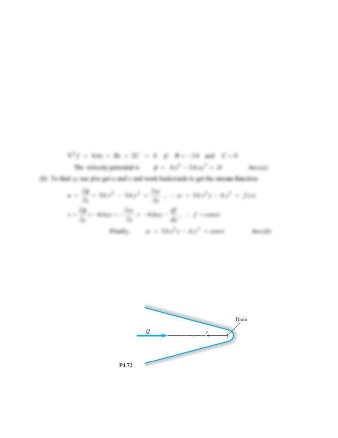
Problem 4.72
Water flows through a two-dimensional narrowing wedge at 9.96 gal/min per meter of width
into the paper. (Fig. P4.72) If this inward flow is purely radial, find an expression, in SI units,
for (a) the stream function, and (b) the velocity potential of the flow. Assume one-dimensional
flow. The included angle of the wedge is 45.
Solution 4.72
3 2 2 , where 0f A x B x y C x D A= + + +
The wedge angle equals /4 radians. At any given position r, the inward flow equals
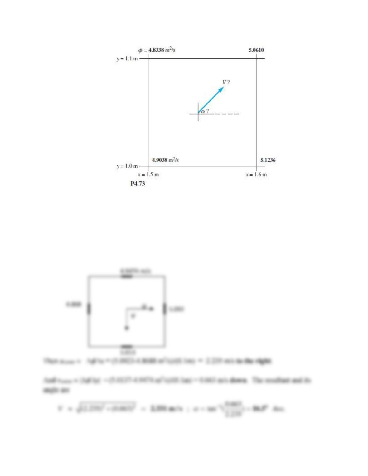
Problem 4.73
A CFD model of steady two-dimensional incompressible flow has printed out the values of
velocity potential
(x, y), in m2/s at each of the four corners of a small 10cm-by10cm cell, as
shown in Fig. P4.73. Use these numbers to estimate the resultant velocity in the center of the
cell and its angle
with respect to the x axis.
Solution 4.73
Quick analysis: the
values are lower on the left than the right, therefore u is to the right. The
values are lower on the top than the bottom, therefore v is down. There are several ways to
estimate the center velocities. One simple way is to compute average values of
on the sides:
Problem 4.74
Consider the two-dimensional incompressible polar-coordinate velocity potential
where B is a constant and L is a constant length scale.
(a) What are the dimensions of B?
(b) Locate the only stagnation point in this flow field.
(c) Prove that a stream function exists and then find the function
(r,
).
Solution 4.74
(a) To give
its correct dimensions of {L2/T}, the constant B must have the dimensions of
velocity, or {L/T}. Ans.(a)
LBrB += cos
Problem 4.75
Given the following steady axisymmetric stream function:
valid in the region 0 r R and 0 z L.
(a) What are the dimensions of the constant B?
(b) Show whether this flow possesses a velocity potential and, if so, find it. (c) What might this flow
represent? HINT: Examine the axial velocity vz.
Solution 4.75
(a) From the definition of
(r, z) in Eqs. (4.105), the dimensions of
are {L3/T}. Thus B has
velocity dimensions, {B} = {L/T}. Ans.(a)
4
2
2
( ) , where and are constants
22
Br
r B R
R
=−
Problem 4.76*
A two-dimensional incompressible flow has the velocity potential
where K and C are constants. In this discussion, avoid the origin, which is a singularity (infinite
velocity).
(a) Find the sole stagnation point of this flow, which is somewhere in the upper half plane.
(b) Prove that a stream function exists and then find
(x, y), using the hint that
dx/(a2+x2) = (1/a)tan-1(x/a).
Solution 4.76*
(a) Find the velocity components and see where they both equal zero:
2 2 2 2
( ) ln( )K x y C x y
= − + +
Problem 4.77
Outside an inner, intense-activity circle of radius R, a tropical storm can be simulated by a polar-
coordinate velocity potential
(r,
) = Uo R
, where Uo is the wind velocity at radius R.
(a) Determine the velocity components outside r = R. (b) If, at R = 25 mi, the velocity is
100 mi/h and the pressure 99 kPa, calculate the velocity and pressure at r = 100 mi.
Solution 4.77
(a) First, convert Uo = 100 mi/h = 44.7 m/s and R = 25 mi = 40,200 m. The velocities are
calculated from
, as requested in Prob. P4.58:
Problem 4.78
An incompressible, irrotational, two-dimensional flow has the following stream function in polar
coordinates:
sin( ) , where and are constants.
n
Ar n A n
=
Find an expression for the velocity potential of this flow.
Solution 4.78
Use
to find the velocity components, then integrate back to find
.
d
Problem 4.79*
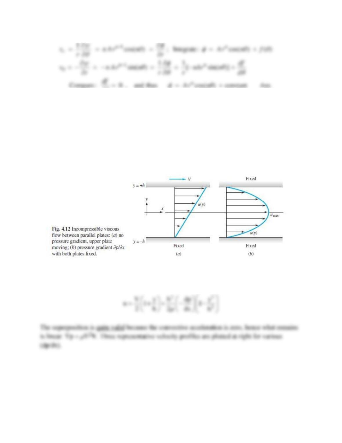
Study the combined effect of the two viscous flows in Fig. 4.12. That is, find u(y) when the upper
plate moves at speed V and there is also a constant pressure gradient (dp/dx). Is superposition
possible? If so, explain why. Plot representative velocity profiles for (a) zero, (b) positive, and
(c) negative pressure gradients for the same upper-wall speed V.
Solution 4.79
The combined solution is
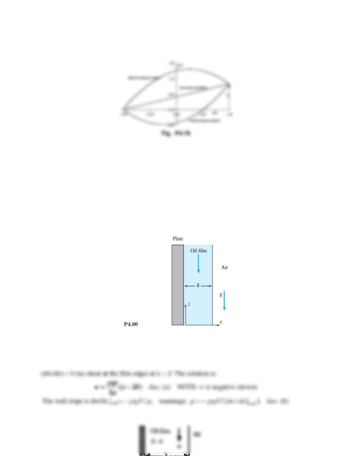
Problem 4.80*
Oil, of density ρ and viscosity μ , drains steadily down the side of a vertical plate, as in Fig. P4.80.
After a development region near the top of the plate, the oil film will become independent of z
and of constant thickness δ . Assume that w = w (x) only and that the atmosphere offers no shear
resistance to the surface of the film. ( a ) Solve the Navier-Stokes equation for w ( x ), and sketch
its approximate shape. ( b ) Suppose that film thickness δ and the slope of the velocity profile at
the wall [ ∂w/∂x] wall are measured with a laser-Doppler anemometer (Chap. 6). Find an
expression for oil viscosity μ as a function of ( ρ , δ , g , [ ∂w/∂x ] wall ).
Solution 4.80
First, there is no pressure gradient
p/
z because of the constant-pressure atmosphere. The
Navier-Stokes z-component is
(d2w/dx2) =
g, and the solution requires w = 0 at x = 0 and
Problem 4.81
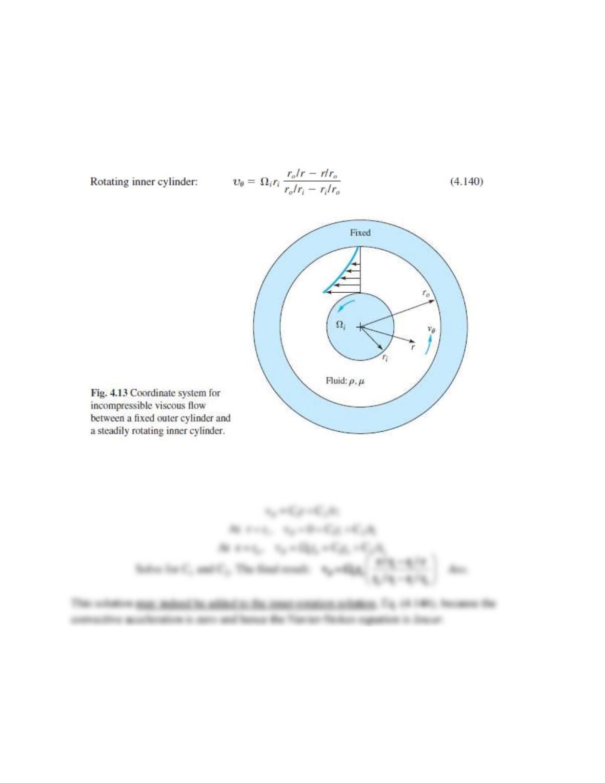
Modify the analysis of Fig. 4.13 to find the velocity v
when the inner cylinder is fixed and the
outer cylinder rotates at angular velocity o. May this solution be added to Eq. (4.140) to
represent the flow caused when both inner and outer cylinders rotate? Explain your conclusion.
Solution 4.81
We apply new boundary conditions to Eq. (4.145) of the text:
Problem 4.82*
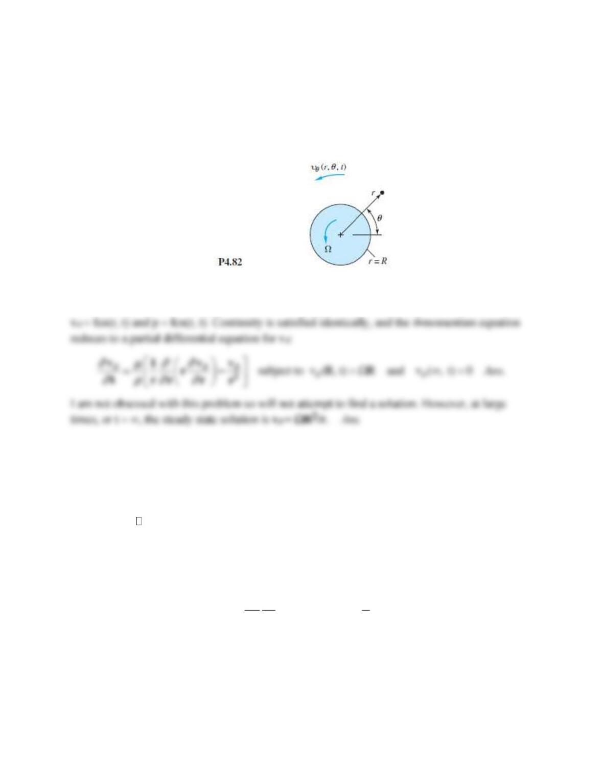
A solid circular cylinder of radius R rotates at angular velocity in a viscous incompressible
fluid which is at rest far from the cylinder, as in Fig. P4.82. Make simplifying assumptions and
derive the governing differential equation and boundary conditions for the velocity field v
in the
fluid. Do not solve unless you are obsessed with this problem. What is the steady-state flow field
for this problem?
Solution 4.82
We assume purely circulating motion: vz = vr = 0 and
/
= 0. Thus the remaining variables are
Problem 4.83
The flow pattern in bearing lubrication can be illustrated by Fig. P4.83, where a viscous oil (
,
)
is forced into the gap h(x) between a fixed slipper block and a wall moving at velocity U. If the
gap is thin,
,hL
it can be shown that the pressure and velocity distributions are of the form
p = p(x), u = u(y),
= w = 0. Neglecting gravity, reduce the Navier-Stokes equations (4.38) to a
single differential equation for u(y). What are the proper boundary conditions? Integrate and
show that
2
1( ) 1
2
dp y
u y yh U
dx h
= − + −
where h = h(x) may be an arbitrary, slowly varying gap width. (For further information on
lubrication theory, see Ref. 16.)
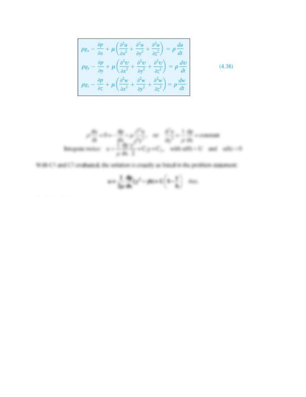
Solution 4.83
With u = u(y) and p = p(x) only in the gap, the x–momentum equation becomes
Problem 4.84
Consider a viscous film of liquid draining uniformly down the side of a vertical rod of radius a,
as in Fig. P4.84. At some distance down the rod the film will approach a terminal or fully
developed draining flow of constant outer radius b, with
z =
z(r),
=
r = 0. Assume that
the atmosphere offers no shear resistance to the film motion. Derive a differential equation for
z, state the proper boundary conditions, and solve for the film velocity distribution. How does
the film radius b relate to the total film volume flow rate Q?
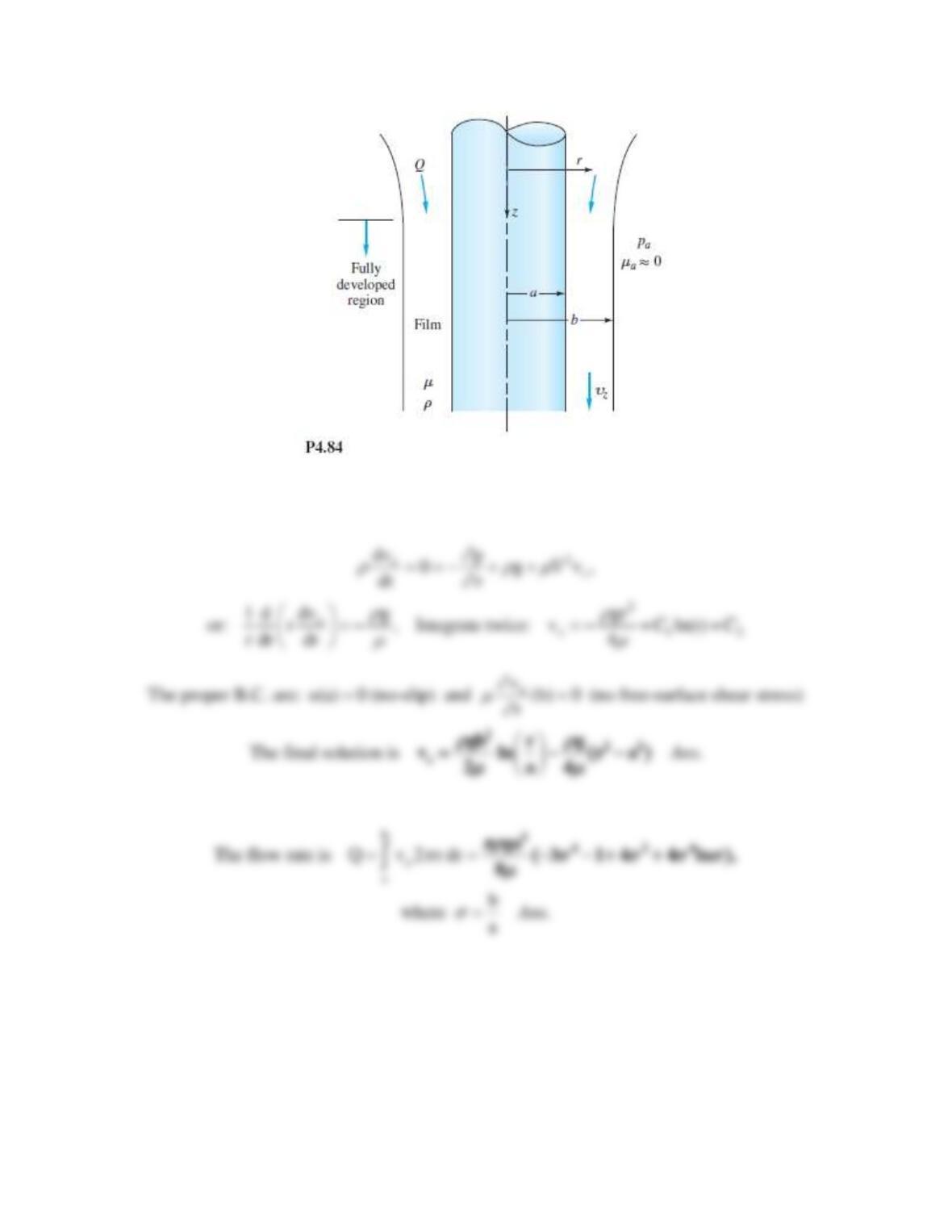
Solution 4.84
With vz = fcn(r) only, the Navier-Stokes z-momentum relation is
Problem 4.85
A flat plate of essentially infinite width and breadth oscillates sinusoidally in its own plane beneath a
viscous fluid, as in Fig. P4.85. The fluid is at rest far above the plate. Making as many simplifying
assumptions as you can, set up the governing differential equation and boundary conditions for
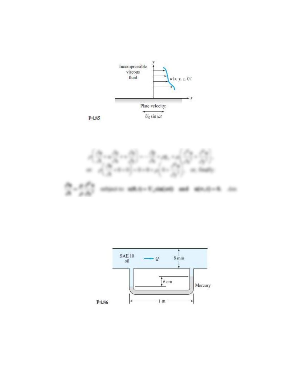
finding the velocity field u in the fluid. Do not solve (if you can solve it immediately, you might be
able to get exempted from the balance of this course with credit).
Solution 4.85
Assume u = u(y, t) and
p/
x = 0. The x-momentum relation is
Problem 4.86
SAE 10 oil at 20C flows between parallel plates 8 mm apart, as in Fig. P4.86. A mercury
manometer, with wall pressure taps 1 m apart, registers a 6-cm height, as shown. Estimate the
flow rate of oil for this condition.
Solution 4.86
Assuming laminar flow, this geometry fits Eqs. (4.143, 144) of the text: