Problem 4.C1
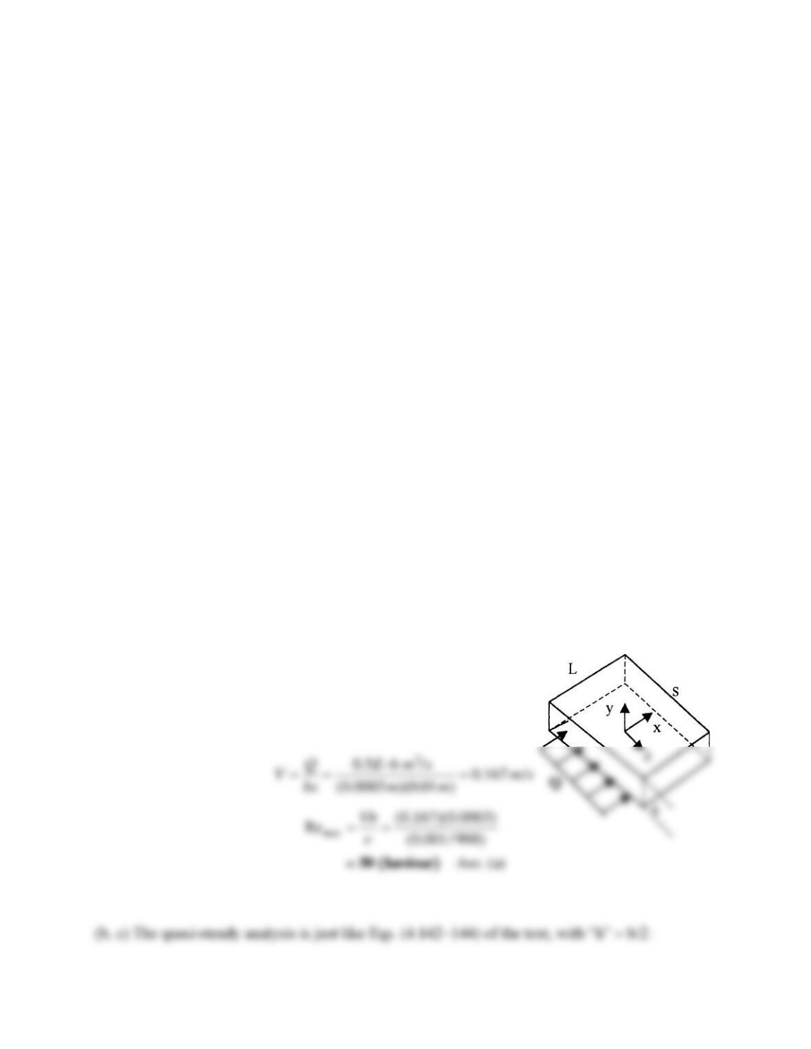
In a certain medical application, water at room temperature and pressure flows through a
rectangular channel of length L = 10 cm, width s = 1.0 cm, and gap thickness b = 0.30 mm. The
volume flow is sinusoidal, with amplitude
ˆ
Q
= 0.50 mL/s and frequency f = 20 Hz, i.e.,
Q =
ˆ
Q
sin(2
f t).
(a) Calculate the maximum Reynolds number (Re = Vb/
)
, based on maximum average velocity
and gap thickness. Channel flow like this remains laminar for Re less than about 2000. If Re is
greater than about 2000, the flow will be turbulent. Is this flow laminar or turbulent?
(b) In this problem, the frequency is low enough that at any given time, the flow can be solved as
if it were steady at the given flow rate. (This is called a quasi-steady assumption.) At any
arbitrary instant of time, find an expression for streamwise velocity u as a function of y, μ, dp/dx,
and b , where dp/dx is the pressure gradient required to push the flow through the channel at
volume flow rate Q . In addition, estimate the maximum magnitude of velocity component u.
(
c
) At any instant of time, find a relationship between volume flow rate Q and pressure gradient
dp/dx . Your answer should be given as an expression for Q as a function of dp/dx, s, b, and
viscosity μ.
(d) Estimate the wall shear stress, τw as a function of
ˆ
Q
, f, μ, b, s , and time (t).
(e) Finally, for the numbers given in the problem statement, estimate the amplitude of the wall
shear stress,
ˆw
, in N/m2.
Solution 4.C1
(a) Maximum flow rate is the amplitude,
Qo = 0.5 ml/s, hence average velocity
V = Q/A:
Problem 4.C2
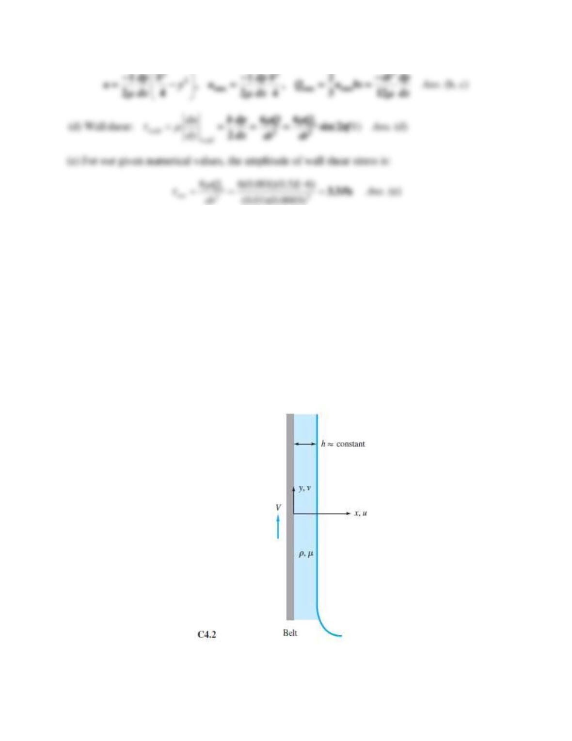
A belt moves upward at velocity V, dragging a film of viscous liquid of thickness h, as in
Fig. C4.2. Near the belt, the film moves upward due to no-slip. At its outer edge, the film moves
downward due to gravity. Assuming that the only non-zero velocity is v(x), with zero shear stress
at the outer film edge, derive a formula for
(a) v(x);
(b) the average velocity Vavg in the film; and
(c) the wall velocity VC for which there is no net flow either up or down.
(d) Sketch v(x) for case (c).
Solution 4.C2
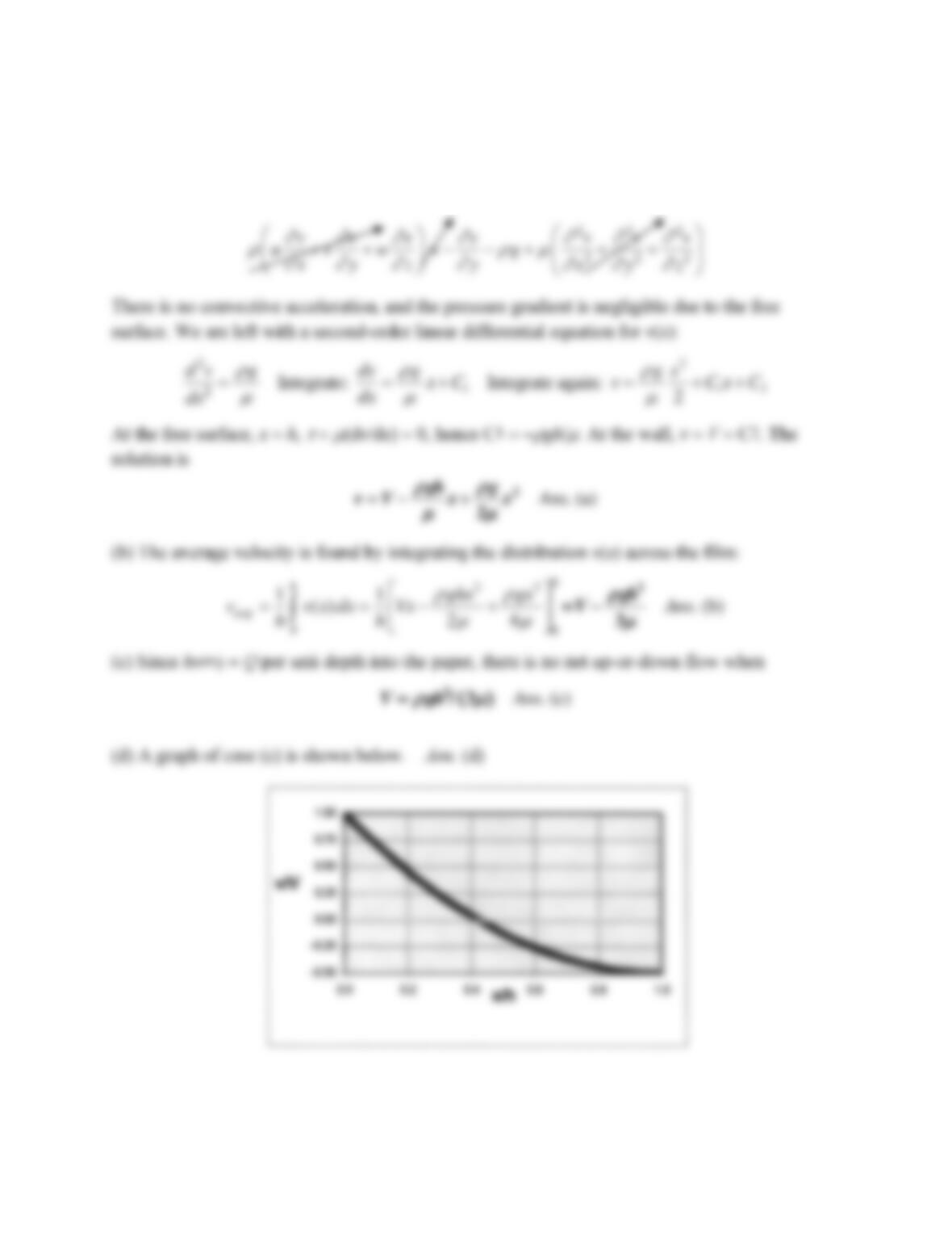
(a) The assumption of parallel flow, u = w = 0 and v = v(x), satisfies continuity and makes the
x– and z-momentum equations irrelevant. We are left with the y-momentum equation:
Problem 4.W1
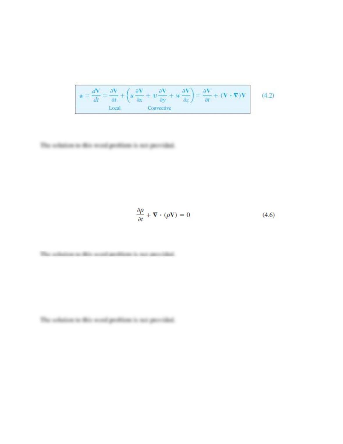
The total acceleration of a fluid particle is given by Eq. (4.2) in the Eulerian[?] system, where V
is a known function of space and time. Explain how we might evaluate particle acceleration in
the Lagrangian[?] frame, where particle position r is a known function of time and initial
position, r = fcn( r0 , t ). Can you give an illustrative example?
Solution 4.W1
Problem 4.W2
Is it true that the continuity relation, Eq. (4.6), is valid for both viscous and inviscid, newtonian
and non-newtonian, compressible and incompressible flow? If so, are there any limitations on
this equation?
Solution 4.W2
Problem 4.W3
Consider a CD (compact disc) rotating at angular velocity Ω . Does it have vorticity in the sense
of this chapter? If so, how much vorticity?
Solution 4.W3
Problem 4.W4
How much acceleration can fluids endure? Are fluids like astronauts, who feel that 5 g is severe?
Perhaps use the flow pattern of Example 4.8, at r = R , to make some estimates of fluid
acceleration magnitudes.
Solution 4.W4
Problem 4.W5
State the conditions (there are more than one) under which the analysis of temperature
distribution in a flow field can be completely uncoupled, so that a separate analysis for velocity
and pressure is possible. Can we do this for both laminar and turbulent flow?
Solution 4.W5
Problem 4.W6
Consider liquid flow over a dam or weir. How might the boundary conditions and the flow
pattern change when we compare water flow over a large prototype to SAE 30 oil flow over a
tiny scale model?
Solution 4.W6
Problem 4.W7
What is the difference between the stream function ψ and our method of finding the streamlines
from Sec. 1.11? Or are they essentially the same?
Solution 4.W7
Problem 4.W8
Under what conditions do both the stream function ψ and the velocity potential ϕ exist for a flow
field? When does one exist but not the other?
Solution 4.W8
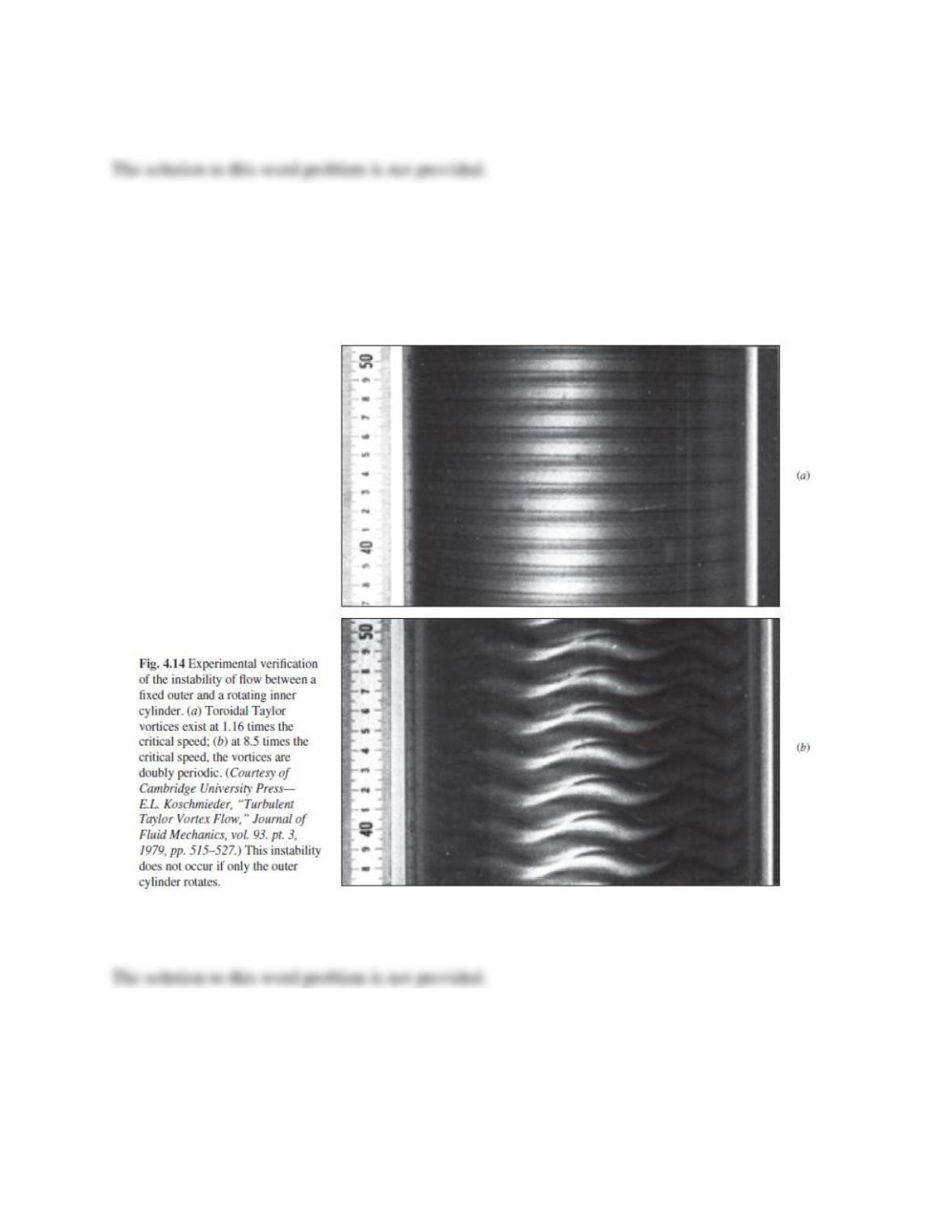
Problem 4.W9
How might the remarkable three-dimensional Taylor instability of Fig. 4.14 be predicted?
Discuss a general procedure for examining the stability of a given flow pattern.
Solution 4.W9
Problem 4.W10
Consider an irrotational, incompressible, axisymmetric ( ∂/∂ θ = 0) flow in (r, z) coordinates.
Does a stream function exist? If so, does it satisfy Laplace’s equation? Are lines of constant ψ
equal to the flow streamlines? Does a velocity potential exist? If so, does it satisfy Laplace’s
equation? Are lines of constant ϕ everywhere perpendicular to the ψ lines?
Solution 4.W10
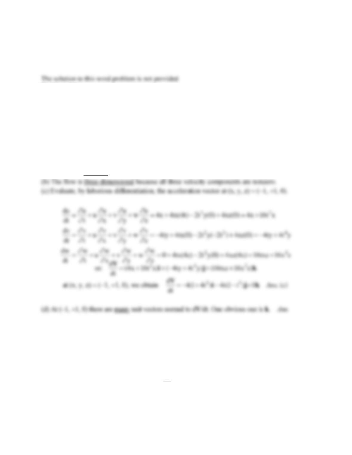
Problem 4.1
An idealized velocity field is given by the formula
2
4 2 4tx t y xz= − +V i j k
Is this flow field steady or unsteady? Is it two- or three-dimensional? At the point
(x, y, z) = (–1, +1, 0), compute (a) the acceleration vector and (b) any unit vector normal to the
acceleration.
Solution 4.1
(a) The flow is unsteady because time t appears explicitly in the components.
Problem 4.2
Flow through the converging nozzle in Fig. P4.2 can be approximated by the one-dimensional
velocity distribution
o
2
1 0 0
x
u V w
L
+
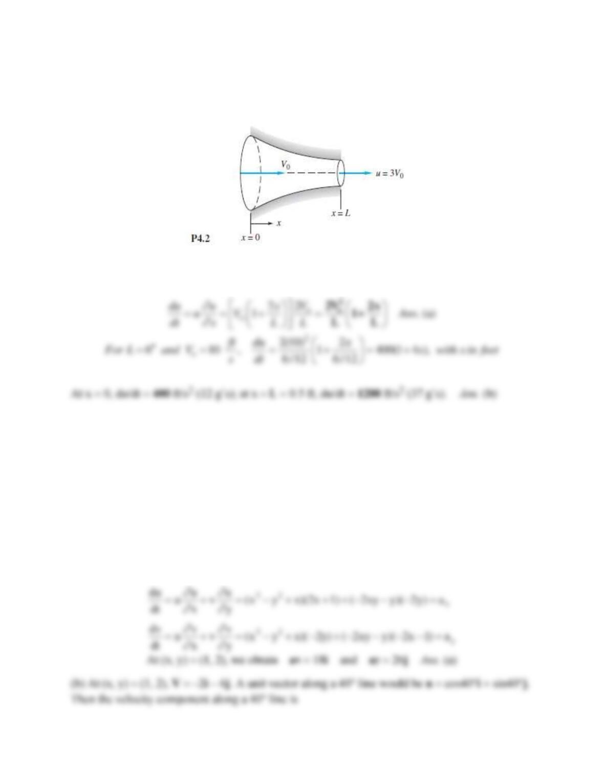
(a) Find a general expression for the fluid acceleration in the nozzle. (b) For the specific case
Vo = 10 ft/s and L = 6 in, compute the acceleration, in g’s, at the entrance and at the exit.
Solution 4.2
Here we have only the single ‘one–dimensional’ convective acceleration:
Problem 4.3
A two-dimensional velocity field is given by
V = (x2 – y2 + x)i – (2xy + y)j
in arbitrary units. At (x, y) = (1, 2), compute (a) the accelerations ax and ay, (b) the velocity
component in the direction
= 40, (c) the direction of maximum velocity, and (d) the direction
of maximum acceleration.
Solution 4.3
(a) Do each component of acceleration:
Problem 4.4
A simple flow model for a two-dimensional converging nozzle is the distribution
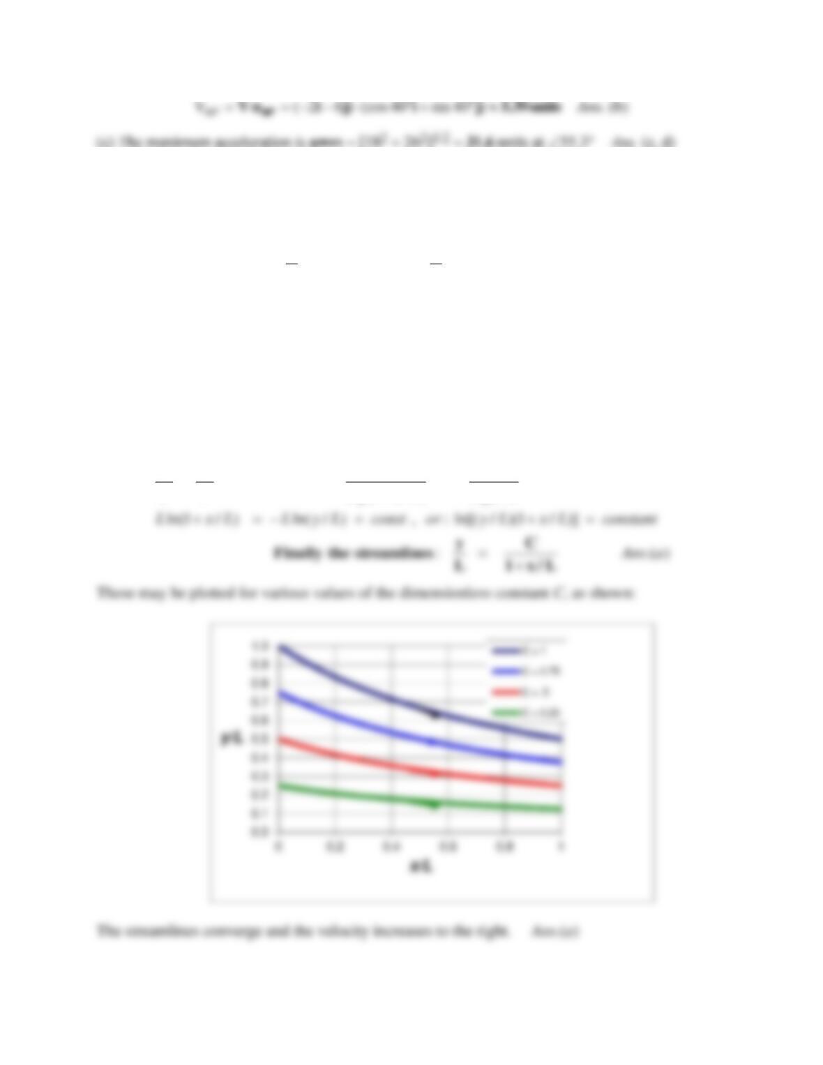
(a) Sketch a few streamlines in the region 0<x/L<1 and 0<y/L<1, using the method of
Section 1.11. (b) Find expressions for the horizontal and vertical accelerations.
(c) Where is the largest resultant acceleration and its numerical value?
Solution 4.4
The streamlines are in the x-y plane and are found from the velocities:
(1 ) 0
oo
xy
u U v U w
LL
= + = − =
:(1 / ) /
o
dx dy dx dy U
u v U x L U y L
= = −
+
or integrate Cancel
Problem 4.5
The velocity field near a stagnation point may be written in the form
oo
o
u v and are constants
U x U y UL
LL
−
==
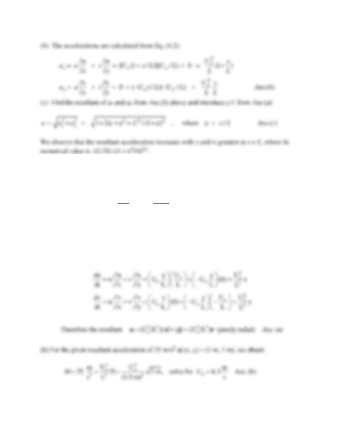
(a) Show that the acceleration vector is purely radial. (b) For the particular case L = 1.5 m, if the
acceleration at (x, y) = (1 m, 1 m) is 25 m/s2, what is the value of Uo?
Solution 4.5
(a) For two-dimensional steady flow, the acceleration components are
Problem 4.6
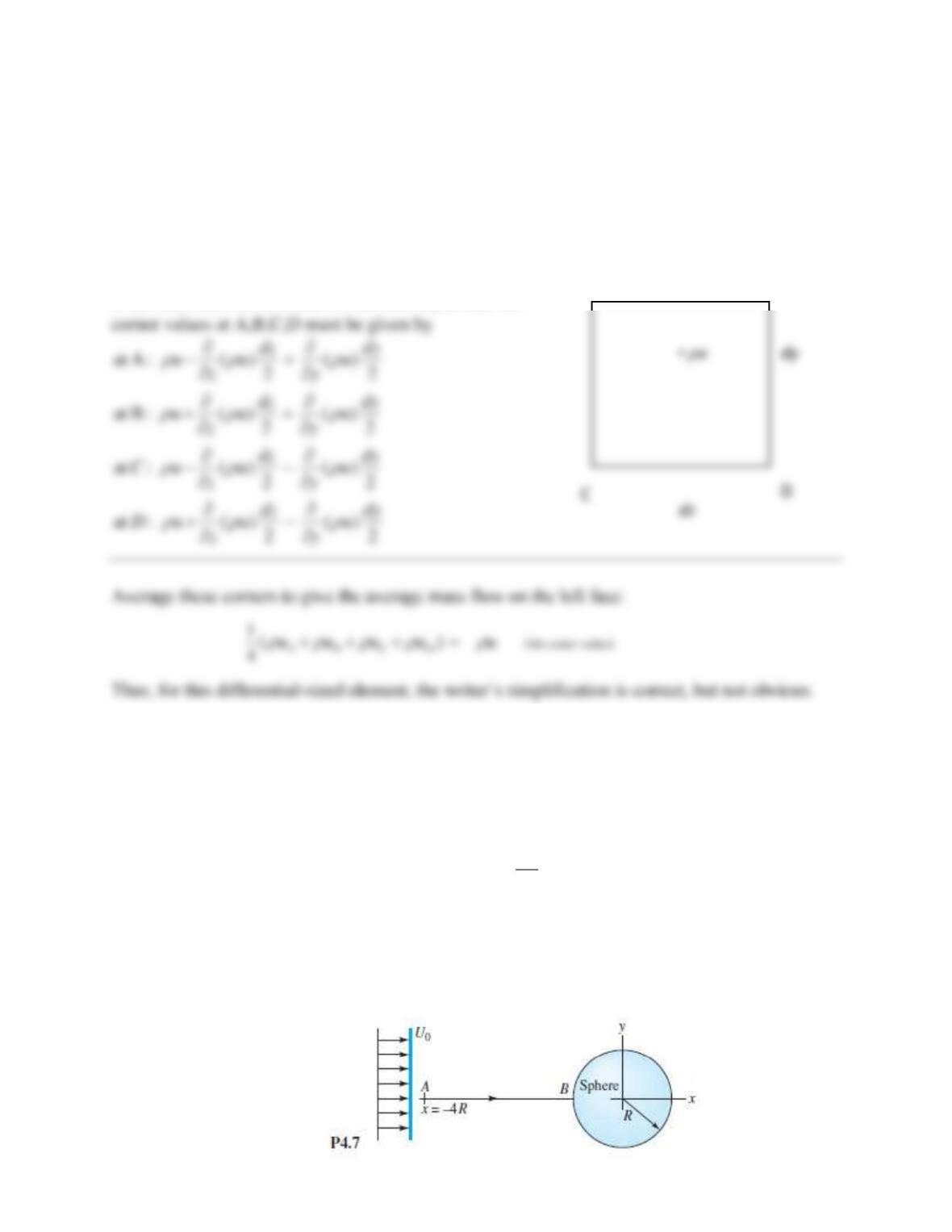
In deriving the continuity equation, we assumed, for simplicity, that the mass flow per unit area
on the left face was just ρu . In fact, ρ u varies also with y and z , and thus it must be different on
the four corners of the left face. Account for these variations, average the four corners, and
determine how this might change the inlet mass flow from ρu dy dz .
Solution 4.6
Consider the sketch at right for the left face. A B
If the mass flow in the center of the face is ρu, then the
Problem 4.7
Consider a sphere of radius R immersed in a uniform stream Uo, as shown in Fig. P4.7. According to
the theory of Chap. 8, the fluid velocity along streamline AB is given by
3
o3
u1
R
Ux
= = +
V i i
Find (a) the position of maximum fluid acceleration along AB and (b) the time required for a fluid particle to
travel from A to B.
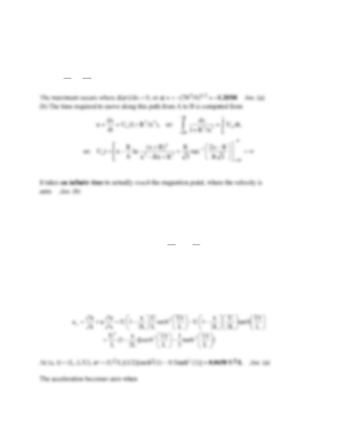
Solution 4.7
(a) Along this streamline, the fluid acceleration is one-dimensional:
3 3 3 4 3 4 3 7
o o o
du u
u U (1 R /x )( 3U R /x ) 3U R (x R x ) for x R
dt x
−−
= = + − = − + −
Problem 4.8
When a valve is opened, fluid flows in the expansion duct of Fig. P4.8 according to the
approximation
1 tanh
2
x Ut
ULL
=−
Vi
Find (a) the fluid acceleration at (x, t) = (L, L/U) and (b) the time for which the fluid acceleration
at x = L is zero. Why does the fluid acceleration become negative after condition (b)?
Solution 4.8
This is a one-dimensional unsteady flow. The acceleration is
Problem 4.9
An idealized incompressible flow has the proposed three-dimensional velocity distribution
V = 4xy2i + f(y)j – zy2k
Find the appropriate form of the function f(y) which satisfies the continuity relation.
Solution 4.9
Simply substitute the given velocity components into the incompressible continuity equation:
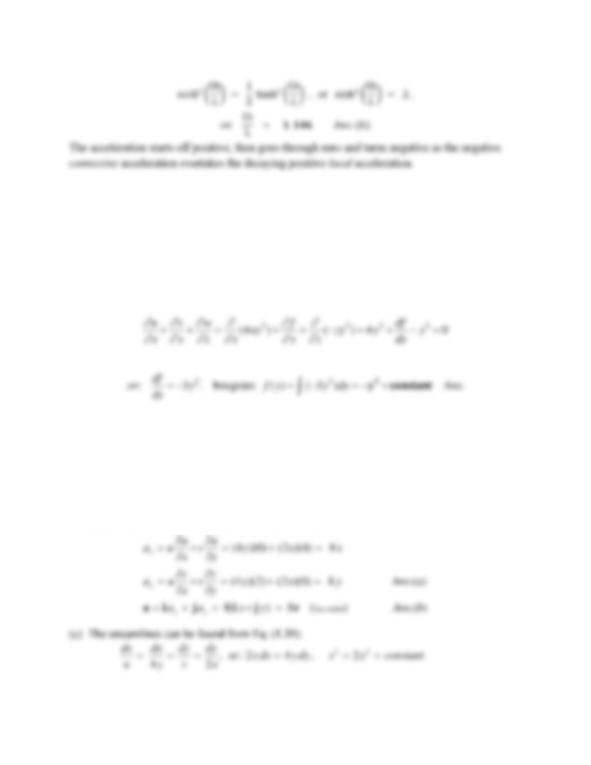
Problem 4.10
A two-dimensional incompressible flow has the velocity components u = 4y and v = 2x.
(a) Find the acceleration components. (b) Is the vector acceleration radial? (c) Sketch a
few streamlines in the first quadrant and determine if any are straight lines.
Solution 4.10
We can use the two-dimensional acceleration formulas:
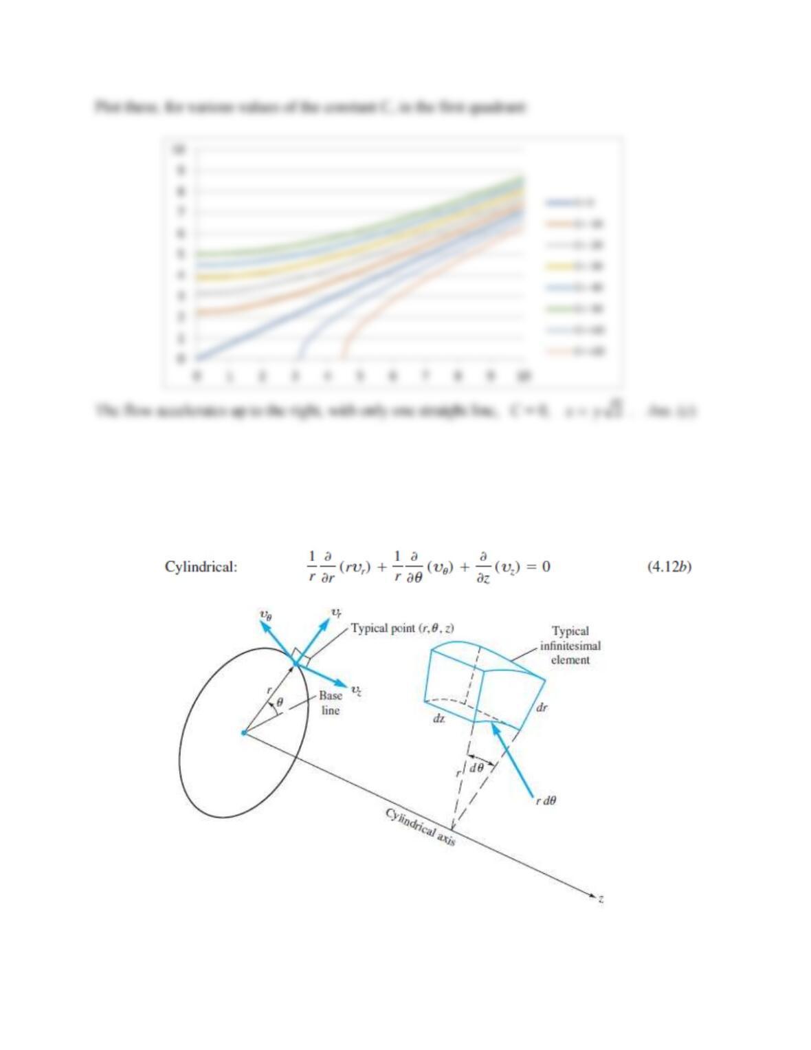
Problem 4.11
Derive Eq. (4.12b) for cylindrical coordinates by considering the flux of an incompressible fluid
in and out of the elemental control volume in Fig. 4.2.
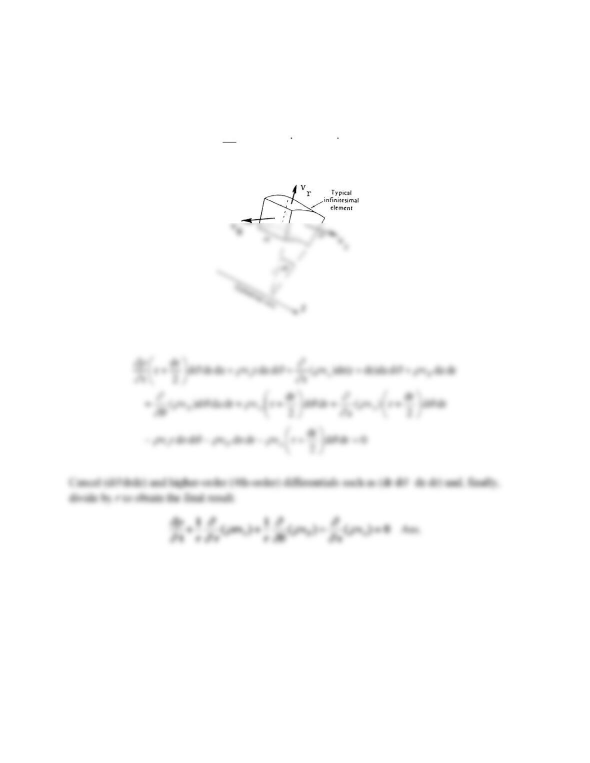
Solution 4.11
For the differential CV shown,
out in
d ol dm dm 0
t
+ − =
Problem 4.12
Spherical polar coordinates (r,
,
) are defined in Fig. P4.12. The Cartesian transformations are
x = r sin
cos
y = r sin
sin
z = r cos
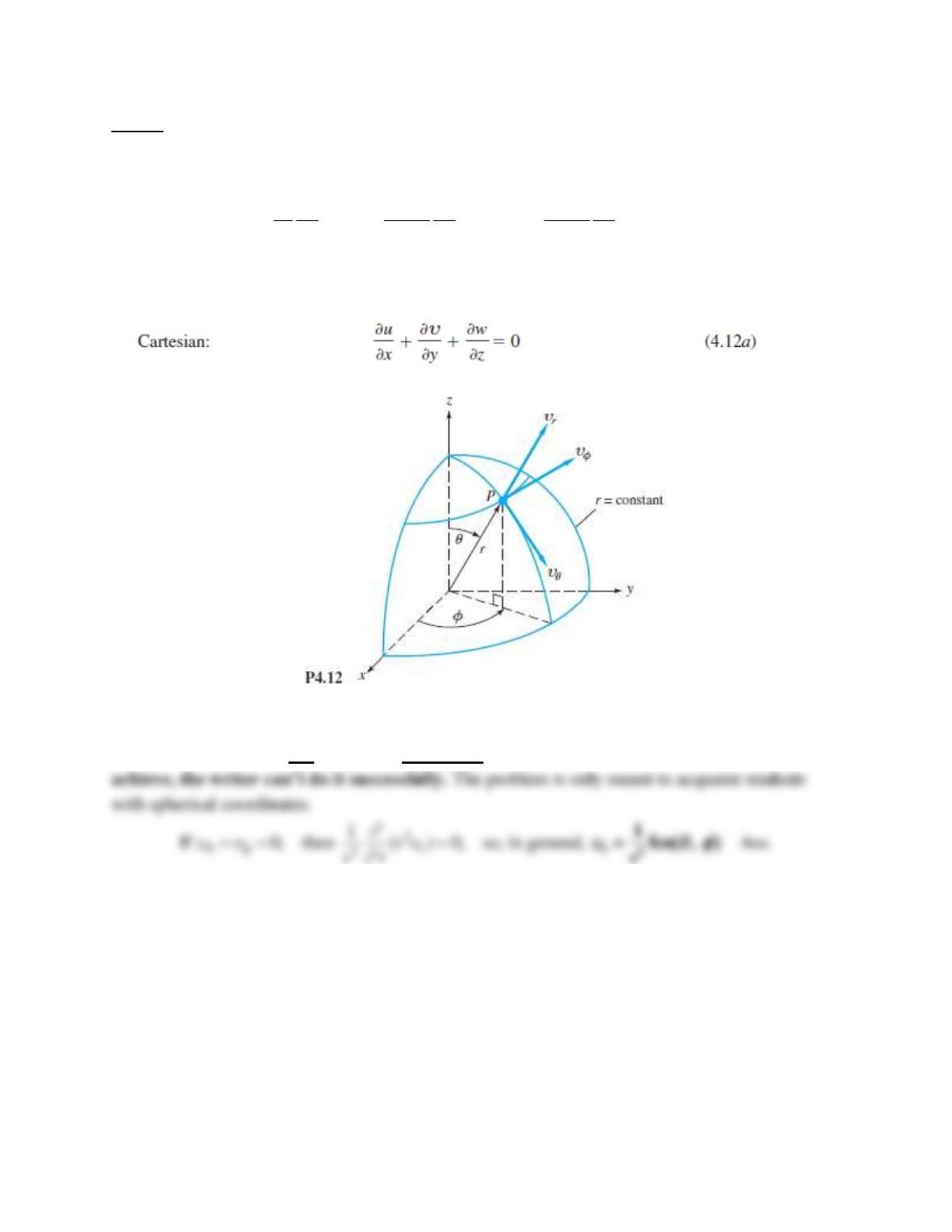
Do not show that the Cartesian incompressible continuity relation [Eq. (4.12a)] can be
transformed to the spherical polar form
2
2
1 1 1
( ) ( sin ) ( ) 0
sin sin
r
r
r r r
r
+ + =
What is the most general form of
r when the flow is purely radial, that is,
and
are zero?
Solution 4.12
Note to instructors: Do not assign the derivation of this continuity relation, it takes years to
Problem 4.13
For an incompressible plane flow in polar coordinates, we are given
32
cos sin
r
v r r
=+
Find the appropriate form of circumferential velocity for which continuity is satisfied.
Solution 4.13
Substitute into continuity, Eq. (4.9), for incompressible flow:
Problem 4.14
For incompressible polar-coordinate flow, what is the most general form of a purely circulatory
motion,
=
(r,
, t) and
r = 0, that satisfies continuity?
Solution 4.14
If vr = 0, the plane polar coordinate continuity equation reduces to:
Problem 4.15
What is the most general form of a purely radial polar-coordinate incompressible flow pattern,
r =
r(r,
, t) and
= 0, which satisfies continuity?
Solution 4.15
If v
= 0, the plane polar coordinate continuity equation reduces to:
Problem 4.16
Consider the plane polar coordinate velocity distribution
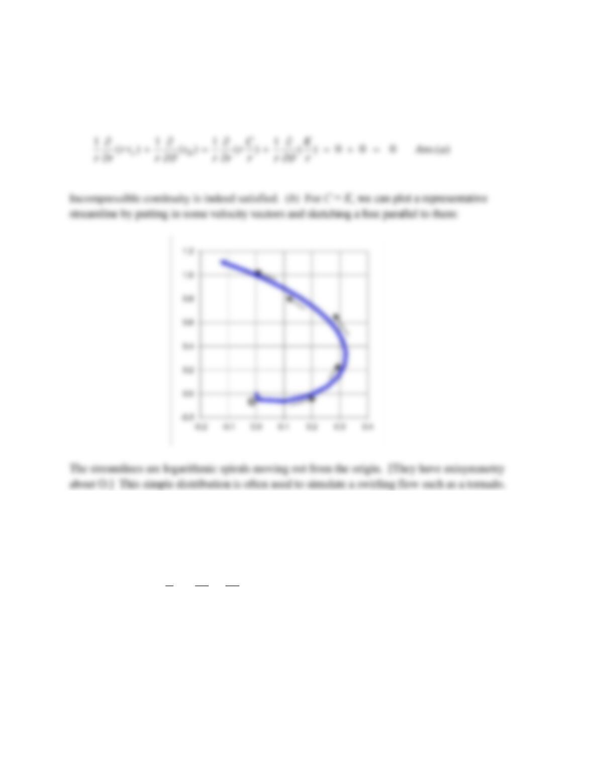
where C and K are constants. (a) Determine if the equation of continuity is satisfied. (b) By
sketching some velocity vector directions, plot a single streamline for C = K. What might this
flow field simulate?
0
rz
CK
v v v
rr
= = =
Solution 4.16
(a) Evaluate the incompressible continuity equation (4.12b) in polar coordinates:
Problem 4.17
An excellent approximation for the two-dimensional incompressible laminar boundary layer on
the flat surface in Fig. P4.17 is
34 1/2
34
2 2 for , where , constant()
y y y
u U y C x C
− + = =
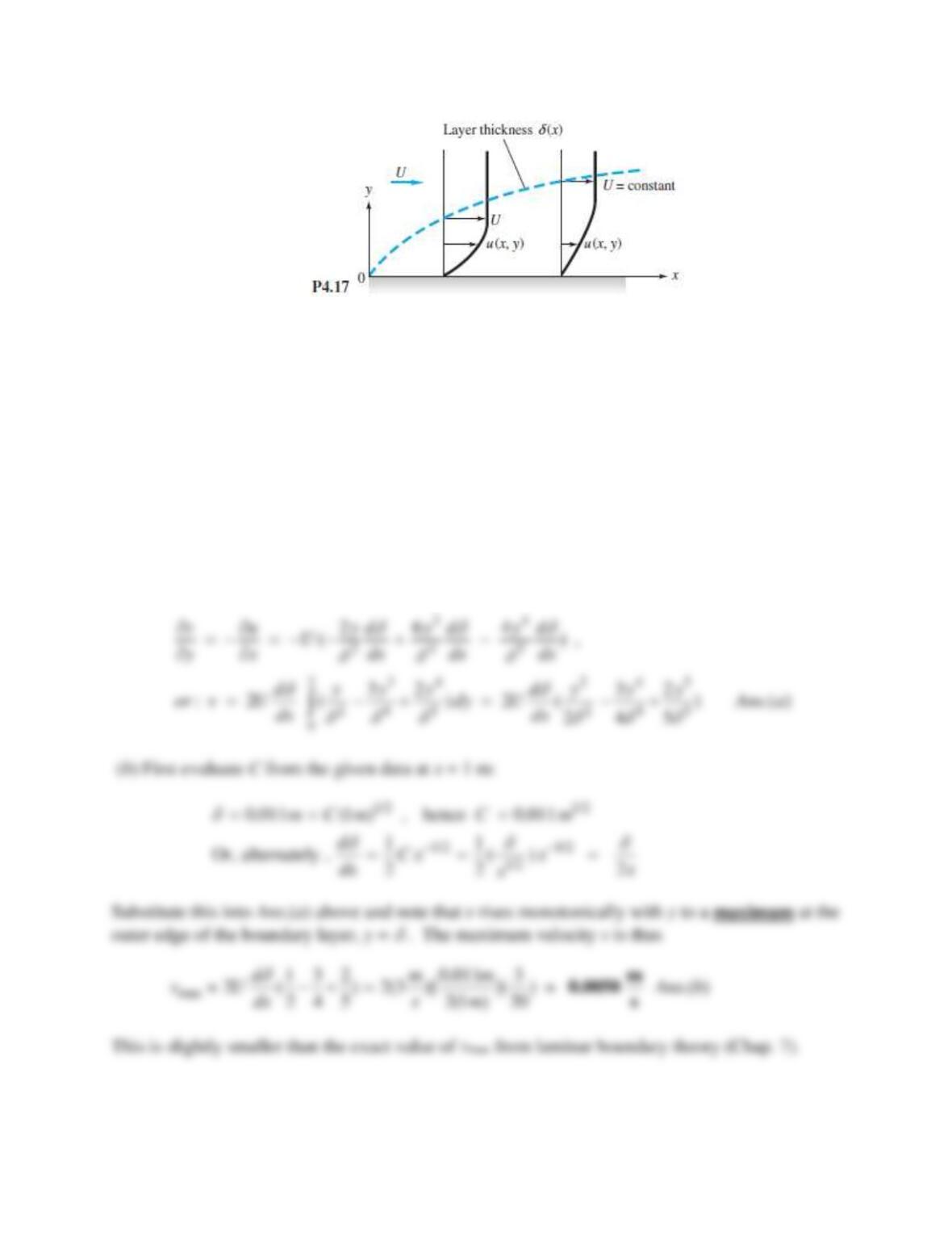
(a) Assuming a no-slip condition at the wall, find an expression for the velocity component
v(x, y) for y
.
(b) Then find the maximum value of v at the station x = 1 m, for the particular case of
airflow, when U = 3 m/s and
= 1.1 cm.
Solution 4.17
(a) With u known, use the two-dimensional equation of continuity to find v:
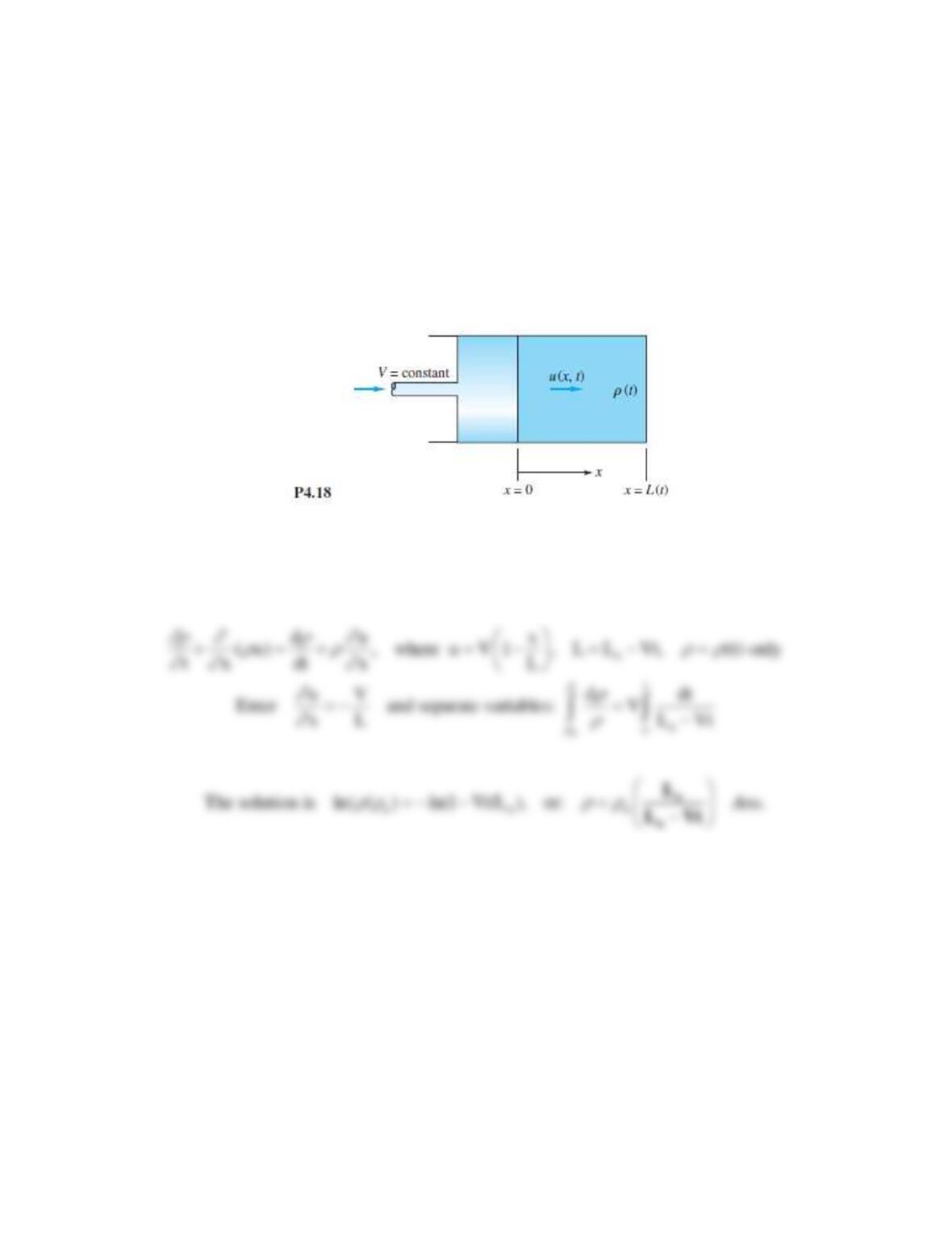
Problem 4.18
A piston compresses gas in a cylinder by moving at constant speed V, as in Fig. P4.18. Let the gas
density and length at t = 0 be
o and Lo, respectively. Let the gas velocity vary linearly from
u = V at the piston face to u = 0 at x = L. If the gas density varies only with time, find an expression
for
(t).
Solution 4.18
The one-dimensional unsteady continuity equation reduces to
Problem 4.19
A proposed incompressible plane flow in polar coordinates is given by
( )
2 cos(2 ) ; 2 sin 2
r
v r v r
= = −
(a) Determine if this flow satisfies the equation of continuity. (b) If so, sketch a possible
streamline in the first quadrant by finding the velocity vectors at (r, θ) = (1.25, 20º), (1.0, 45º),
and (1.25, 70º). (c) Speculate on what this flow might represent.
Solution 4.19